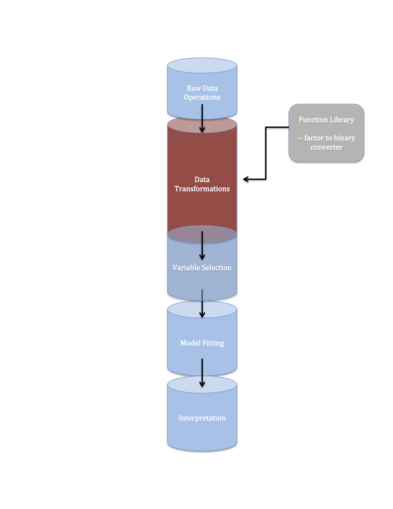
Data pipelines 2 data transformations

I was kind of hoping to have a full data pipeline/machine learning pipeline in Python post ready for today. This was to be a companion to the data pipeline in R illustration I posted last week. I fell a little short so I’m settling for shorter, more focused post on an important element of any data pipeline: data transformations.
Side note: I also really wanted to shift gears a little and start playing with data from the Internet Movie Database…but I don’t quite have the necessary Python package installations sorted out yet.
Problem Statement
I have a factor variable that takes say 10 different value and, for the purposes of analysis, I would like to create a set 10 binary/dummy variables. This is a reasonably common task in machine learning and data analysis
More specifically, in this application, I have data on movies. These data include the Title of the Movie, genres to which the movie was assigned, and the text string for the Studio’s movie overview. The overarching question is,
can we train a machine learner to classify movies into the correct genre based on the words in the movie overview?
This post focuses on an important intermediate task for this analysis: representing the words in a movie’s overview as inputs in a data matrix.
Problem Illustration
I’m going to work with a small sample of movie data because I don’t have my data scraper totally polished yet. If you want these data go here.
movie.db <- read.csv('movie_info.csv')
str(movie.db)
'data.frame':	24 obs. of  3 variables:
 $ Title : Factor w/ 24 levels "A Few Good Men",..: 3 19 22 2 4 21 24 8 5 23 ...
 $ Info  : chr  "A live-action adaptation of Disney's version of the classic tale of a cursed prince and a beautiful young woman who helps him b"| __truncated__ "After being bitten by a genetically altered spider, nerdy high school student Peter Parker is endowed with amazing powers." "Set in the 22nd century, The Matrix tells the story of a computer hacker who joins a group of underground insurgents fighting t"| __truncated__ "When three overworked and under-appreciated moms are pushed beyond their limits, they ditch their conventional responsibilities"| __truncated__ ...
 $ Genres: Factor w/ 19 levels "Action, Crime, Thriller",..: 16 17 2 8 11 8 3 11 7 1 ...

 #this is kind of a mess, let's look at few things column-wise to get the flavor of the
 # data
 movie.db$Title
 [1] Beauty and the Beast         Spider Man                   The Matrix
 [4] Bad Moms                     Brides Maids                 The Hangover
 [7] The X-Men                    How to lose a guy in 10 days Despicable Me
[10] The Transporter              Joe Dirt                     Good Will Hunting
[13] Rainman                      A Few Good Men               Jerry Maguire
[16] Milk                         Sideways                     The Big Lebowski
[19] Fargo                        Rio                          Madagascar
[22] Ice Age                      Shrek                        Love Actually

movie.db$Genre[movie.db$Title=='Bad Moms']
[1] Comedy

movie.db$Info[movie.db$Title=='Bad Moms']
[1] "When three overworked and under-appreciated moms are pushed beyond their limits, they ditch their conventional responsibilities for a jolt of long overdue freedom, fun, and comedic self-indulgence."
What I want to do with these data in order to eventually use them to train a machine learner is to:
- split the movie info character string into individual words
- represent each movie as a combination of binary variables (one for each unique word in the combined data set) according to whether or not each word appears in the movie’s info or not.
Problem Solution
Python has kind of a neat way of doing this: with the function CountVectorizer in the scikit-learn module. For now I’m going to stick to R and hopefully switch over to Python for next week’s (planned) 3rd installment of Pipeline posts.
The R Package tidytext has two functions that are supremely useful for what I want to do here:
-
tidytext::unnest_tokens(), which splits a string of text into individual tokens. A token can be defined a lot of ways but for now it’s good enough to think of tokens as the individual words in a text string.
-
tidytext::tf_idf(), which calculates the term frequency-inverse document frequency. This is quantity that is meant to convey how important a word or token is in a particular text.
library(tidytext)
library(dplyr)

#Term Frequency-Inverse Document Frequency------------------

# a couple of nested steps here:

#1. use unnest_token to split the string of words in the column 'Info' into
#    individual words
#2. count the instances of each word in each movie Title
#3. use the bind_tf_idf() function from the tidytext package to
#    get the term frequency inverse document frequency for each
#     Title/word pair.

book_words <- movie.db %>%
  unnest_tokens(word, Info) %>%
  count(Title, word, sort = TRUE) %>%
  group_by(Title) %>%
  mutate(total.words = n_distinct(word)) %>%
  mutate(term.freq=n/total.words) %>%
  bind_tf_idf(word, Title, n) %>%
  ungroup()
#-------------------------------------------------

# get a dictionary of unique words in the full data set
bag.of.words <- c(unique(book_words$word[book_words$tf_idf>0.01 & book_words$tf_idf<0.95]))

# for each movie title form a vector of 0's and 1's according to whether each title
# does or does not contain each word in bag.of.words
X <- matrix(unlist(lapply(unique(movie.db$Title),function(i){
  as.numeric(bag.of.words %in% book_words$word[book_words$Title==i])
})),nr=length(unique(movie.db$Title)),nc=length(bag.of.words))

#coerce to data frame
X <- data.frame(X)

#name columns
names(X) <- bag.of.words

dim(X)
[1]  24 692

X[1:3,26:36]
  at get he's ransom small lambeau level professor when 10 about
1  0   0    0      0     1       0     0         0    0  0     0
2  0   0    0      0     0       0     0         0    0  0     0
3  0   0    0      0     0       0     0         0    0  0     0
>
Here we can see that we have successfully created an input matrix with 24 rows (the number of movie titles in our data set) and 692 columns (1 for each unique word in the original movie introduction columns).
I can’t really print out a 24 X 692 data frame but just printing the first 3 rows and columns 26-36 we can see that this input data frame is just a collection of variables indicating whether certain words appeared in each movie’s info.
Bonus plot
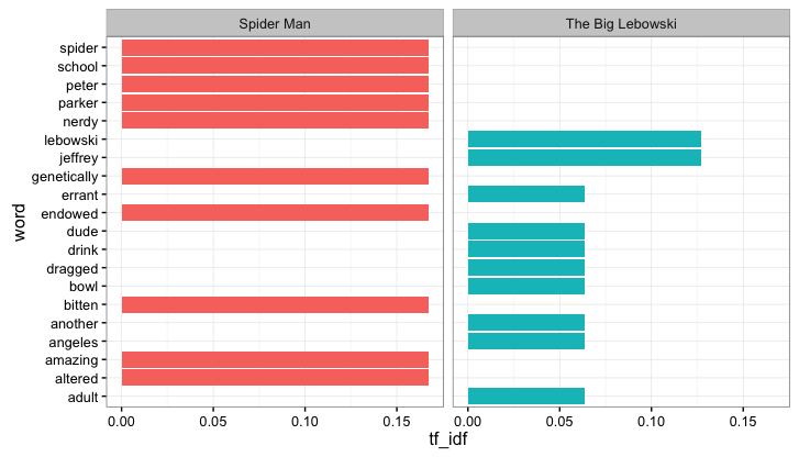
As a final step let’s just display some of the most important words for a couple movies. This won’t be all that informative but I don’t know if I could live with myself if I pushed out a blog post with no plots.
#--------------------------------------------------
# as a final step let's just display the top 3 words
# in terms of tf-idf for each film


top3 <- book_words %>% group_by(Title) %>%
        arrange(-tf_idf) %>% mutate(rank=row_number()) %>%
        filter(rank<=10)

ggplot(subset(top3,Title%in%c('Spider Man','The Big Lebowski')),
       aes(x=word,y=tf_idf,fill=Title)) + geom_bar(stat='identity') +
     facet_wrap(~Title) + coord_flip() + theme_bw() + guides(fill=FALSE)

#-------------------------------------------------

Like I said not super informative. One issue here is that the term frequency-inverse document frequency metric is a lot more powerful when you have a large corpus of words. Note that, for Spider Man, there are lots of words with the same tf-idf…this is because there are lots of words that appear in the description of the movie Spider Man, and appear there more than once, and that don’t appear in any other movie description. If I had more movies (and hence more words) in my data, we could get a better sense of what words are truly unique to a movie or movie genre.
Resources
I found a really cool Python movie data scraping example here. However, I use Anaconda Python I haven’t quite sorted out how to get the TMBD API manager (tmdbsimple) loaded up on my instance of Python. Still, you should check this out, it’s way cool.
There is also a nice tutorial on the use of R’s tidytext here.
I also have a few blog posts where I dealt with some text mining functionalities, give those a look.
Also, I’m pulling movie data from TMBD. You can go here if you want to verify that my data have been correctly input.
