
Machine learning pipelines part 1
To follow along with this post hop over to GitHub and clone my abalone-age repo.
This series of posts was inspired by a cool functionality I found in Python’s SciKitLearn module called Pipeline.
Conceptually, pipeline (in the parlance of data science) refers to the chaining together of a series of tasks (e.g. acquiring data, cleaning data, fitting a model, interpreting the model) to complete some analysis. Specifically, the sklearn.pipeline class in Python provides a cool looking wrapper to combine a bunch of the tasks involved in good empirical work into a few chunks of code.
Here is what I’m scheming to cover in the next few posts:
- some introductory words on data pipelines/machine learning pipelines and reproducible research in general
- an example of an old-school ‘end-to-end’ pipeline in R
- an example of a machine learning pipeline in Python using the sklearn.pipeline class
Preamble
I’m still not sure I feel about the word/concept of pipelines at it used (abused?) by data scientists. On the one hand I like the promotion of a tight, organized workflow that automates data acquisition, data cleaning, modeling, and interpretation in an integrated environment. On the other hand I’m not totally sure we need a new word for this. I mean “building an end-to-end pipeline” is really just another way of saying “doing good reproducible research.” The creation and use of the jargon “pipeline”, “data pipeline”, and “machine learning pipeline” kinda feels like another thing (reproducible research) data science is trying to steal from the research community and pass off like they invented it.
Since culture doesn’t give a shit what I think about it, let’s move on.
What is a pipeline
I’m sure everyone has thier own preferred definition of a data pipeline but I think it’s best defined as a workflow that integrates all the major tasks involved with producing good empirical analysis AND - this is the critical part to me - creating a framework where meta parameters (should we log to dependent variable? should we use 5-fold cross-validation, should we use mean squared error or mean absolute error) can be tested and experimented with.
pipelines are particularly useful concepts for dealing with streaming data
If data are static then any reasonably organized set of scripts should suffice to make the analysis reproduceable. But when one is dealing with data that update on regular intervals and the analysis should be updated with the data, having an organized pipeline is probably really valuable.
pipelines are particularly useful for pure atheoretic machine leaning applications
In classic machine learning applications like spam identification there generally isn’t a lot of debate over which features ought or ought-not to be included in an analysis. The combination of features/inputs that produce the best out-of-sample predictions should be kept and others should be discarded.
This is somewhat different from many science/research applications where the effect of an input may be of particular interest. In these types of cases, there is generally a greater need for human intervention in the model selection process.
Automated pipelines will generally yield more natural benefits for cases requiring minimal human intervention in the model selection process.
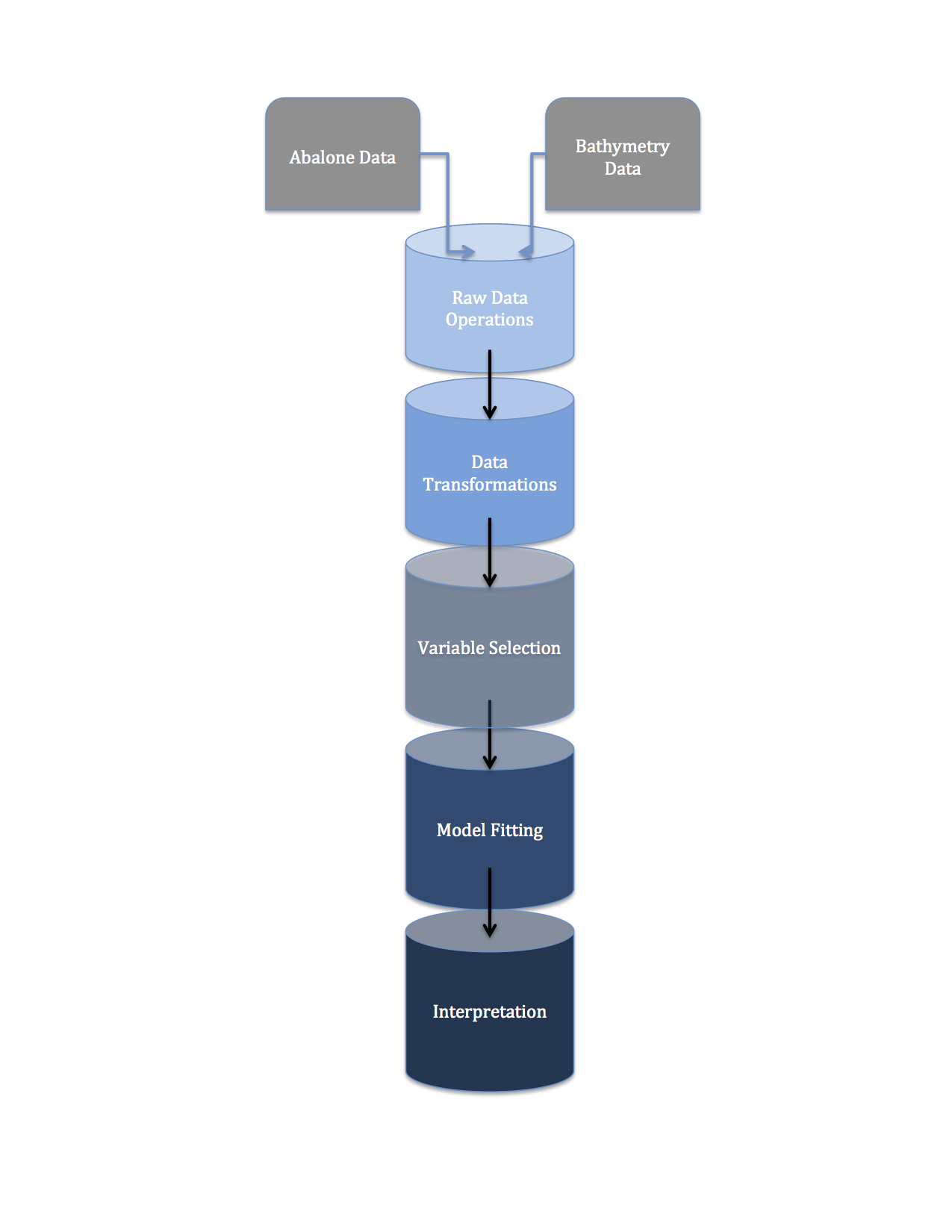
My R Data Pipeline
Before delving into Python’s pipeline() functionalities from the SciKitLearn library, I’m going to illustrate my understanding of a machine learning pipeline with an admittedly ghetto R example.
-
data_prep.R is a script that pulls data from a remote repository, joins it with some static data and prepares the data for analysis.
-
transforms_fn.R is a script that includes some data transformation functions.
-
estimation.R is a script that contains intermediate code to fit some models to data and use cross-validation techniques to determine the best flavor of those models.
-
model.R is the face of our ‘pipeline’. It sequentially: updates the raw data, does some minimal cleaning, invokes some transformation functions to prepare the data for model fitting, estimates 2 classes of model, then compares them using cross-validation.
In the next couple subsections I’ll comment on each of the ‘pipes’ in my pipeline briefly:
Problem Statement
One can read about the boring, tedious nature of trying to infer the age of abalone from the number of rings on it’s shell here. The basic problem is that aging abalone is labor intensive and it would be really cool if there were a way to ‘learn’ an abolone’s age from some easily observable characteristics rather than spending an hour in a lab every time you want to age an abalone.
My example below deals with fitting a non-parametric machine learning model (classification and regression trees) and a parametric regression model to some abalone data in order to develop a model to predict age from observable stuff like weight, shell diameter, etc.
The Data Pull
My experience thus far tells me that pipelines as an analytical concept are likely to be most valuable when one has streaming data that feeds into some analysis and that analysis needs to be updated frequently when new data comes in.
For that reason I choose to work with some data hosted on a remote site. While these data are actually static and are hosted on the UCI Machine Learning Database, since the code is just pinging a URL it’s pretty easy to see how this structure could apply to streaming data where the URL is dynamic.
Also, in the world I live in we generally don’t get all the data we want in one spot. We often have to merge our data of interest with auxiliary information like weather, interest rates, population sizes, or the average wing-span of the African Swallow. For this reason I have chosen to pretend like we also have lat/long coordinates of where each abalone sample was taken. I do this in order to introduce the auxiliary variable: bottom depth.
Bottom depth comes from a topology data layer pulled from ERDDAP. These bottom depths are gridded in regular lat/long intervals. To get bottom depth at the specific lat/long coordinates of our abalone data I include a little routine to use Inverse Distance Weighted Spatial Interpolation.
rm(list=ls())
# load the library
library(RCurl)
library(rerddap)
# specify the URL for the Abalone data CSV
urlfile <-'https://archive.ics.uci.edu/ml/machine-learning-databases/abalone/abalone.data'
# download the file
downloaded <- getURL(urlfile, ssl.verifypeer=FALSE)
# treat the text data as a steam so we can read from it
connection <- textConnection(downloaded)
# parse the downloaded data as CSV
abalone <- read.csv(connection, header=FALSE)
# preview the first 5 rows
head(abalone)

names(abalone) <- c('sex','length','diameter','height','whole_weight','shucked_weight','viscera_weight','shell_weight','ring')

#--------------------------------------------------------------------
# not a real part of the analysis but I'm going to add a totally made up
# location field so we can illustrate a data join in the first
# pipe of our pipeline

lat <- c(rep(39,1000),rep(38.975,1000),rep(38.85,1000),rep(38.5,1177))
long <- c(runif(min=-123.94,max=-123.72,n=1000),
          runif(min=-123.93,max=-123.725,n=1000),
          runif(min=-123.9,max=-123.65,n=1000),
          runif(min=-123.59,max=-123.225,n=1177))
abalone$lat <- lat
abalone$long <- long
#--------------------------------------------------------------------


bathy <- read.csv('data/bathy.csv',skip=1)
names(bathy) <- c('lat','long','meters')

#=====================================================================
# get bottom depths for each observation
library(gstat)
library(sp)
library(maptools)
library(dplyr)

#format the abalone locations
abs.locs <- abalone %>% mutate(x=long,y=lat) %>% select(x,y)
coordinates(abs.locs) = ~x+y

#form the bounding box
bb.lats <- c(max(abalone$lat)+0.04,min(abalone$lat)-0.04)
bb.longs <- c(min(abalone$long)-0.04,max(abalone$long)+0.04)

depths <- tbl_df(bathy) %>%
          filter(lat < bb.lats[1]) %>%
          filter(lat > bb.lats[2]) %>%
          filter(long > bb.longs[1]) %>%
          filter(long < bb.longs[2])

depths <- depths %>% mutate(x=long,y=lat) %>% select(x,y,meters)
coordinates(depths) = ~x+y

idw <- idw(formula=meters~1,locations=depths,newdata=abs.locs)
tmp <- data.frame(idw)
#=====================================================================

#add bottom depths to the abalone data
abalone <- data.frame(abalone,tmp$var1.pred)
names(abalone) <- c('sex','length','diameter','height','whole_weight','shucked_weight',
                    'viscera_weight','shell_weight','ring','lat','long','depth_meters')
saveRDS(abalone,"data/abalone.RDA")
So that’s Step 1: pull the abalone data from the internet, read in the static data on ocean bottom depths, interpolate values and merge data sets so that bottom depth is now included in our data of interest.
Data Tranformation
Researchers, Scientists, Data Scientists, and Empiricists of pretty much all stipes generally have to monkey around with the variables in their data sets a fair amount:
- log transform certain variable to squash their variance
- convert units of measure to other units of measure
- normalize input data (especially popular for artificial neural network models)
- turn some continuous variables in categorical variables
- turn some character variables (months of the year) into binary (0,1) variables.
Most of us do this in a kind of hacky way that involves adding a bunch of columns onto an existing data set.
As near as I can tell, a cool philosophical element to the idea of creating a ‘pipeline’ is that these transformations should be considered meta-parameters on your model and you want to try and engineer your analysis in way that you can easily iterate over these meta-parameters for model selection or sensitivity analysis.
library(dplyr)

#a function to convert depth from meters to fathoms
depth.to.fathoms <- function(var.name,df){
  idx <- which(colnames(df)==var.name)
  df$depth_fm <- df[,idx]*0.54
  return(df)
}


#a function to transform a continuous variable to a categorical one
continuous.to.factor <- function(var.name,cuts,df){
  names <- names(df)
  ncats <- length(cuts)-1
  df$cat <- cut(df[,which(colnames(df)==var.name)],cuts,labels=1:ncats)
  names(df) <- c(names,paste(var.name,"_","cat",sep=""))
  return(df)
}
My transformation function script is pretty short - just two functions that operate over selected columns of the raw data.
Model Estimation
This step involves a little working backward. Basically, I know I want my pipeline to look something like:
pull data –> clean data –> fit model to data –> interpret results
and in the end I want one script that makes it crystal clear how, in what order, and subject to what parameter assumptions each of these steps is carried out.
I know that I don’t want my final script cluttered with lots of different calls to regression functions and the like. I also know that I’m going to fit two models to my abalone data:
-
A non-parametric classification tree
-
A parametric poisson regression
And, for this exercise, I’m going to compare the various models using cross-validation of out-of-sample forecasts.
So my estimation script is going to include a bunch of wrappers to internal R functions that run these two types of model. It’s also going to include some wrappers to the predict() family of functions, which will be the backbone of my cross-validation exercise.
library(tree)


#===================================================
treeclass.est <- function(df){
  ab.tree <- tree(factor(ring)~.,data=df)
  return(ab.tree)
}

model.prune <- function(tree.obj,prune){
  ab.prune <- prune.tree(tree.obj,best=prune)
  return(ab.prune)
}
#=================================================


#=================================================
#Poisson estimator
poisson.fn <- function(y.name,x.name,data){
  formula <- paste(y.name,"~",paste(x.name, collapse='+'))
  poi.reg <- glm(paste(formula),data=abalone,family='poisson')
  return(poi.reg)
}

#=================================================

#================================================
#Cross Validation Functions
cvtree.fn <- function(train.pct,data,best,formula){
  train.idx <- sample(1:nrow(data),train.pct*nrow(data))
  train.df <- data[train.idx,]

  test.df <- abalone[-train.idx,]
  model <- tree(paste(formula),data=train.df)
  pruned.tree <- prune.tree(model,best=best)

  y.hat <- predict(pruned.tree,test.df,type="class")

  pct.correct <- sum(as.numeric(test.df$ring==y.hat))/nrow(test.df)
return(pct.correct)
}


#cross validate the poisson regressions
cvpoi.fn <- function(y.name,x.name,data,train.pct){

  train.idx <- sample(1:nrow(data),train.pct*nrow(data))
  train.df <- data[train.idx,]
  test.df <- abalone[-train.idx,]

  poi.model <-  poisson.fn(y.name=y.name,x.name=x.name,data=train.df)
  y.hat <- round(predict(poi.model,test.df,type='response'),digits=0)
  pct.correct <- sum(as.numeric(test.df$ring==y.hat))/nrow(test.df)

  return(pct.correct)
}
#================================================
Finally, The Pipeline
The script model.R provides a clean interface to my analytical pipeline. It:
-
sources the transformation and estimation functions
-
gets the primary data
-
passes the primary data through some variable transformation operations
-
estimates some models
-
cross-validates models
rm(list=ls())
library(dplyr)
library(data.table)

#----------------------------------
source('functions/transform_fns.R')
source('functions/estimations.R')
#----------------------------------

#----------------------------------
#get data
abalone <- readRDS('data/abalone.RDA')
#----------------------------------

#----------------------------------
# transform data

abalone <- depth.to.fathoms(var.name='depth_meters',df=abalone)

abalone <- continuous.to.factor(var.name='lat',cuts=seq(38,39.06,by=0.06),df=abalone)
#----------------------------------

#----------------------------------
#model data

model1 <- treeclass.est(df=abalone)
size <- summary(model1)$size

#cross-validate some tree-based classifiers
tree.results <- data.frame(rbindlist(lapply(c(0:3),function(i){
   term.nodes <- size - i
   pct.correct <- cvtree.fn(formula=paste("factor(ring)~."),best=term.nodes,
                            train.pct=0.8,data=abalone)
   return(data.frame(tree_size=term.nodes,pct.correct=pct.correct))
})
))
tree.results

  tree_size pct.correct
1         5   0.2392344
2         4   0.2488038
3         3   0.2177033
4         2   0.1949761

#find the best poisson model
x <- list(c('shell_weight','diameter'),c('shell_weight','diameter','lat'),
          c('shell_weight','diameter','sex'))

poi.results <- data.frame(rbindlist(lapply(c(1:3),function(i){
  x.name <- x[[i]]
  pct.correct <- cvpoi.fn(y.name='ring',x.name=x.name,data=abalone,train.pct=0.8)
  return(data.frame(poi.model=i,pct.correct=pct.correct))
})
))
poi.results

  poi.model pct.correct
1         1   0.1614833
2         2   0.1674641
3         3   0.1961722
#----------------------------------
At the end of it all here’s what I did:
-
Trained a classification tree algorithm to learn abalone age from a swath of observable characteristics.
-
The best tree size was found to be 5 terminal nodes. I compared the default tree to pruned trees with 1, 2, 3, and 4 terminal nodes. The 4 node tree actually provided more correct out-of-sample predictions
-
The I ran 3 different poisson regressions to predict abalone age. The 3 models were distinguished by their combination of input variables.
-
Using cross-validation techniques, I evaluated the poisson models. I found that the tree-based classifiers provided more correct out-of-sample predictions than the poisson regression.
Quick Wrap-up
This R pipeline isn’t the best and does have some idiosyncrocies but I like it. As an analyst I sometimes don’t pay as much attention as I should to things like variable selection/model selection, variable transformation, etc. It’s not that I don’t do these things, it’s just that I sometimes do them in a more ad-hoc manner than I should.
The concept of a pipeline seems especially valuable to me if it motivates one to organize their work in a way that allows easy examination of some meta-parameters like:
- what if used the square-root transform of the response variable instead of the log transform?
- what if I categorized time of day (morning, afternoon, night) rather than use a continuous measure?
- what if I used 5-fold Cross Validation instead of 10-fold?
- what if I included different combinations of input variables in the Poisson regression?