My first post on this topic was pretty rushed.

There is a lot that goes into doing a half decent sentiment analysis both mechanically and analytically. Like a lot of my post I’m a little more concerned with getting you guys up and running (and hopefully able to start your own learn-by-doing process) quickly…With that goal in mind, I’m leaving the heavy lifting (relative strength and weakness of Naive Bayes v. Support Vector Machine v. insert favorite ensemble classifier here) to somebody else and focusing mainly on how to:

1. get some data you might want

2. train a naive bayes classifier, and

3. use the trained algorithm to classify tweets as positive v. negative

Background 1: Resources

For this post I borrowed heavily from a great post by Laurent Luce. There were a number of other blog posts that I got some helpful nuggets from:

• http://chengjunwang.com/en/2012/03/sentiment-analysi-with-python/
• https://marcobonzanini.com/2015/03/02/mining-twitter-data-with-python-part-1/
• http://mark-kay.net/2013/12/18/collecting-tweets-using-python/

These were all really good resources…for my Python knowledge level, I found them all lacking in some small ways. I’ve tried to fill in those gaps with my post.

Background 2: Motivation

This little exercise (along with my early post of scrapping from Twitter) is mainly focused on a conceptually simple idea: can we use data from Twitter to determine whether, on net, people have a positive or negative view of the National Oceanic and Atmospheric Administration? Admittedly, this is a little campy. It’s probably a lot more important (or at least more potentially profitable) for businesses and brands to gauge public opinion about themselves then it is a government science agency. However, the basic concept of knowing whether people think we are doing a good job or a shitty one is still somewhat important. And beyond the little toy example I set up here, Sentiment Analysis can probably be leveraged to address other important issues along the lines of, “how to communicate science effectively to the public”…which is something that is a very important part of NOAA’s mission.

Spoiler Alert: I’m not actually going to provide a satisfying answer to the motivating question, “do people think we are doing a good job.” However, maybe some of the tools I’m providing here will motivate some industrious young researcher to follow-up with a better analysis than I’m about to shit out here.

Background 3: Naive Bayes Classifier

There is no shortage of reputable resources for learning about Naive Bayes classification. I enjoyed the mix of practicality, mathematical rigor, and conciseness available here…but ‘the Google’ abounds with free and accessable introductions to Naive Bayes classification.

Like many things I discuss here there is a lot of nuance to the Naive Bayes text classifier that I encourage you to flush out on your own. The 2 cent version of the classifier goes something like this:

Bayes’ Rule says that,

The basic philosophy of Bayesian decision making is that one has:

1. a prior expectation about the probability of an event: It typically rains 20 days out of 30 days in November in Portland

2. a piece of data: the weather man predicts rain today

3. a likelihood: the weather man predicts rain 50% of the time that it actually rains.

The object of Bayes’ Rule is to combine prior expectation with data and a likelihood to update one’s subjective expectation about an outcome. This updated expectation is the posterior probability…in the case above,

To finish this with a numerical example we need an additional piece of data: the likelihood the weather man predicts rain when it does not rain (let’s call this 30%)…then the posterior (updated probability) of rain today given that it is November in Portland and the weatherman predicts rain is,

…that is we started out thinking that there was a 67% chance of rain but after we observed the weatherman’s prediction we updated our expectation to 76%.

Let’s now consider a more relevant and concrete example: classifying a newly viewed tweet as either positive or negative.

I’m going to rewrite Bayes’ Rule with a notation I like a little better. Let,

• \(x\) be the tweet
• \(c\) be the possible classifications \(c_{1} and c_{2}\) corresponding to ‘positive’ and ‘negative’ respectively.
• \(x_{i}\) be the features of \(x\)…if you want to get away from the ML jargon for right now just think of ‘features’ as the words in a tweet. In more general applications they don’t need to be limited to just the words but if the abstractness of ‘features’ is giving you heartburn just replace it ‘words.’

The posterior probability that a tweet is positive given the content of the tweet can be written as an application of Bayes’ Rule:

Let’s make this slightly more concrete and suppose that the tweet we are looking to classify is ‘NOAA sucks.’ Here, the feature of the tweet are

In the simplest possible application of the Naive Bayes Classifier we are going to classify this tweet as positive if,

Let’s illustrate by calculating,

There are three parts to this posterior probability:

\(P(c_{1})\), the prior probability

\(P(x)\), the evidence

Class Conditional Probability

A key, and sometimes considered limiting feature of Naive Bayes Classifiers is the assumed conditional independence of features. In our case this basically means that observing the feature “NOAA” in a tweet does not make it any more or less likely that we will encounter the feature “sucks.” It’s pretty easy to imagine possibile violation of this assumption (observing ‘peanut’ in a text string makes it much more likely one will also encounter ‘butter’ in that same string) but as a matter of empirics Naive Bayes has been shown to work pretty well so we’re just gonna roll with it for now.

The cool thing about conditional independence is that it makes things really simple,

and these individual likelihoods can be estimated from frequencies,

where the numerator is just the number of occurrences of $x_{1}$ in $c_{1}$ and the denominator is total number of features in $c_{1}$.

The Prior

Bayes’ Rule combines a prior expectation with a likelihood to form the posterior probability. Here the prior is the unconditional probability of observing a positive tweet,

We can again estimate this from frequencies,

The Evidence

The denominator in Bayes’ Rule is the unconditional probability of observing the data \(P(x)\). In our case, this is just like asking what is the probability of observing a tweet with features “NOAA” and “sucks” in our data sample. This probability can be calculated,

but doesn’t really need to be. It doesn’t need to be evaluated because our decision rule is:

if \(P(c_{1}|x)>P(c_{2}|x)\),

then, classify \(x\) as positive.

The decision rule for a positive classification can be rewritten,

Writing it this way we can see that the denominator is the same on both sides of the inequality and hence won’t affect the classification.

To put it in very oversimplified terms: the Naive Bayes Classifier,

• observes the features (in our case these will be words but in more general applications they could be other stuff too) of a bunch of tweets.
• observes the classification of those tweets.
• based on the frequencies of features in tweets labeled ‘positive’ or ‘negative’, it calculates the probabilities that a new tweet with certain features is either positive or negative.
• finally, based on that probability it classifies a tweet as ‘positive’ or ‘negative’

I know I’ve said it like 3 times already but I’m gonna say it again: good content analysis/sentiment analysis/whatever is complicated and there is lot more to it than just finding a big box of words labeled ‘positive’ and ‘negative’ and then pushing the magic button that classifies new word combinations. I’m giving you the really unsophisticated version because my main concerns are:

1. giving a simple but quasi-realistic example so you can start to try and imagine how you might want to use a content/sentiment analysis, and

2. provide some code that is again simple but not trivial so you get quickly get a sentiment analysis going…then poke around inside the routines to see what’s happening and get a deeper understanding of the topic by picking it apart from the inside.

Step-by-Step

Ok, now that we’ve dispensed with a small introduction on Naive Bayes Classification, here are the mechanics to performing a Twitter Based Sentiment Analysis in Python:

Step 1: Set up the training data

The ultimate goal here is to have an algorithm capable of looking at a tweet involving the key phrase ‘NOAA Fisheries’ and tell if the tweet is positive or negative in sentiment. We are going to use the Naive Bayes Classifier. In order to apply that method to our ‘NOAA Fisheries’ tweets we need to teach it what a positive tweet looks like and what a negative tweet looks like.

Step 1A: Get classified tweets

One of the keys to a decent text classifier is getting a set of pre-classified text that the algorithm can ‘learn’ from. If one were so inclined, I suppose one could sit around for hours pulling tweets, looking at them, classifying them as positive or negative, and saving the results. I’m am not so inclined….mostly because I’m sure it would take forever.

In order for an algorithm to learn how to classify

• Thanks NOAA for protecting marine mammals (positive)

and possibly being able to differentiate it from

• Thanks NOAA for establishing bycatch limits for GoM…12 years too late (negative)

it needs to see lots of different combinations of the keywords (‘thanks’,’NOAA’,’protecting’,’marine’,’mammals’,’bycatch’,’too’).

Luckily, there appear to be a few publicly available data sets with hundreds of thousands classified tweets. I used a dataset available from the University of Michigan but you can google “Twitter Sentiment Analysis Corpus” and probably come up with other options if you don’t like this one.

I downloaded the data into a .csv file. Here I’m going to read in this data file and subset it.

#training data
import pandas as pd
import nltk
import numpy as np
import random

training_tweets = pd.read_csv('/Users/aaronmamula/Documents/Python projects/sentimentanalysis/Sentiment Analysis Dataset.csv')
training_tweets['sent'] = np.where(training_tweets['Sentiment']==0, 'negative', 'positive')

#it is taking way too long to train this classifier using all 
# 1 million training tweets...I'm going to subset the data
rows = random.sample(training_tweets.index, 10000)

training_tweets=training_tweets.ix[rows]

Quick note on the subsetting: I tried training the Naive Bayes Classifier on the full list of ~2 million pre-classified tweets. It ran for like an hour and still wasn’t done…so I killed it and culled the training data down to (what I thought was) a manageable but still realistic training set of 100,000 tweets.

Update: even cutting the training set down to 100,000 took forever…so I cut it again to 10,000. Even that took 15 minutes to train. Most of that I believe is due to inefficiencies that I am responsible for (I’ll talk about these at the end).

Step 1B: Massage the training set

Basically what I need to do here is to extract the features of training set. To do that I’m going to:

1. subset the dataframe containing the pre-classified tweets and keep only 2 columns: the content of the tweet and the classification.

2. convert the subsetted data frame into a list of tuples

3. Remove punctuation

4. coerce all the text to lower case just for consistency and efficiency (I don’t want our classifier to try and learn the difference between “Cool” and “cool.”

5. remove common stop words…here I’m just going to remove words less than 3 letters (a, he, of, etc)

#----------------------------------------------------------------
#1 & #2. subset the training set and convert it to a list of tuples

training_set=training_tweets[['SentimentText','sent']]
tuples=[tuple(x) for x in training_set.values]
#-----------------------------------------------------------------

#-----------------------------------------------------------
#3, #4, & #5: 
#convert everything to lowercase and remove common stop words
# that are shorter than 3 characters...also remove 
# punctuation...this might not be optimal in the long-run
# but at them moment I'm anticipating a lot of problems
# with punctuation in our training set

tweets = []
for (words, sentiment) in tuples:
    words_filtered = re.sub('[^A-Za-z0-9]+', ' ', words)
    words_filtered = [e.lower() for e in words_filtered.split() if len(e) >= 3]
    tweets.append((words_filtered, sentiment))
#-----------------------------------------------------------

Basically what I’ve done here is taken a data frame that had tweets stored as a single string entry in one column and a classification (‘positive’ or ‘negative’) in another column and

1. turned it into a list of lists where the first element of the first list is the string entry for tweet #1 and the second entry in the first list is the classification…and the first element in the second list is the string entry for tweet #2 and the second element of the second list is the classification for tweet #2, etc, etc.

2. then I took the first element of each list (which is a string of text) and

• parsed it into a list where each word in the original text string is an element in the list.
• threw out punctuation and special characters
• threw out words less than 3 letters in length (common stop words like ‘a’, ‘an’, ‘he’, etc).

Step 1C: Extract features

So now I have the list of tweets set up the way I want, the next step is to create the inputs that the NLTK module in Python needs in order to do the classification.

def get_words_in_tweets(tweets):
    all_words = []
    for (words, sentiment) in tweets:
      all_words.extend(words)
    return all_words

def get_word_features(wordlist):
    wordlist = nltk.FreqDist(wordlist)
    word_features = wordlist.keys()
    return word_features

word_features = get_word_features(get_words_in_tweets(tweets))

def extract_features(document):
    document_words = set(document)
    features = {}
    for word in word_features:
        features['contains(%s)' % word] = (word in document_words)
    return features

Here is something worth spending a few lines on: our feature extractor here basically creates a dictionary of all the words used in our training set… When we pass a tweet to the feature extractor it is going to compare the context of that tweet to every entry in it’s dictionary…

In our training set there are A LOT of slang words and A LOT of proper nouns like Twitter Handles. I’m guessing I could make the classifier a lot more efficient by removing Twitter Handles from the training dictionary. I don’t think these add much to the ability to correctly identify sentiment.

Step 2: Train the Classifier

Finally, we train the classifier:

#this creates a set of T/F entries for every tweet in the training
# set.  The T/F outcomes indicate which features contained in the 
# training set are present in each training tweet

training_set = nltk.classify.apply_features(extract_features, tweets)

#Let's have a look at this traning_set object...it's too big to print
# to the console so I'll print it to a text file and open in an editor

import json

t1=training_set[1]
t1=t1[0]

# save to file:
with open('/Users/aaronmamula/Documents/Python projects/sentimentanalysis/my_file.json', 'w') as f:
    json.dump(t1, f)

The object training_set is a tuple with each entry corresponding to a tweet in the training data. The first element of each tuple is a dictionary containing every word in the training set and a T/F indicator for whether that word was found in the tweet. The second element of the tuple is the classification.

If we look at the second tweet (still getting used to the 0 indexing in Python so I naturally use 1 as my default first index) in the training data:

we see it has the word ‘doing’

In [309]: tuples[1]
Out[309]: ('@DavidArchie i WISH you were doing a Toronto show on tour ', 'negative')

For illustrative purposes I’ve dumped the element from the object ‘training_set’ corresponding to this tweet from the training data into a text file so you can get an idea of what the ‘training_set’ object looks like:

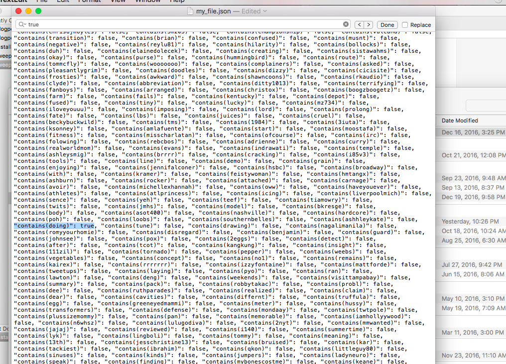
Notice that, if you look very close, you can see the line

“contains(doing): true”…surrounded by a bunch of “contains(otherwords): false.”

Perhaps the complexity of text classification was/is readily apparent to everyone else…it wasn’t really until I looked under the hood at some of these feature extractors that realized the scale of this type of operation. The screen shot above is an entry for A SINGLE TWEET in the training data…and there are over a million tweets in the training data.

Now the fun stuff, we actually train the classifier:

#now for some real black box shit:

tic = time.clock()
classifier = nltk.NaiveBayesClassifier.train(training_set)
toc = time.clock()
toc - tic

Out[265]: 908.8567419999999

Step 3: Apply the trained classifier

Once the Naive Bayes Classifier is trained, it is ready to receive input in the form of new tweets to classify. This is where our earlier twitter scraping comes in. We pass our list of a few hundred tweets mentioning @NOAA Fisheries to the classifier and we get back the modeled sentiment (‘positive’ or ‘negative’) of each tweet.

#first a trivial one just to see if things pass the sniff test:

tweet = 'Larry is my friend'
	...print classifier.classify(extract_features(tweet.split()))
positive

So now I’m going to try this out on one of the actual tweets that I pulled [in my last post using tweepy to interface with Twitter (https://aaronmams.github.io/Sentiment-Analysis-1-Twitter-Scraping-with-Python/). I intentionally picked a difficult tweet in order to demonstrate some conceptual hurdles with Sentiment Analysis and text classification. The parsed tweet looks like this:

“Under reported fish catch is a serious issue that has to be addressed Kenneth Sherman from NOAAFisheries LME18 https t co zXJX2JHgov”

#finally try the classifier out on the NOAA tweets...
# row 91 in the noaa_tweets is a good reference tweet 

noaa_text = noaa_tweets['tweet']
testtweet=noaa_text[91]

testtweet
'"Under-reported #fish catch is a serious issue that has to be addressed", Kenneth Sherman from @NOAAFisheries #LME18 https://t.co/zXJX2JHgov'

#parse it           
testtweet = re.sub('[^A-Za-z0-9]+', ' ', testtweet)       

#split it
print classifier.classify(extract_features(testtweet.split()))
negative

Our test tweet from the data set of all tweets with an @NOAAFisheries mention is a difficult one to classify as positive or negative because it’s not really either of those. This brings up a few complications with Sentiment Analysis that occured to me while I was doing this:

1. There is a lot of content related to NOAA Fisheries that is news-related. It’s neither positive nor negative but just a statement of fact: “NOAAFisheries establishes new rules for mitigating sea turtle bycatch in the Gulf of Mexico” or “NOAA Fisheries estimates spawning stock biomass of purple delicious fish declined.” I’m not really sure what, if anythign to do about this.

2. Related to number 1 above, there is a lot of content involving NOAA Fishieres on Twitter that is simply people sharing a weblink and mentioning @NOAAFisheres. I suspect I could establish more sophisticated filters when pinging Twitter for data that would solve this problem (if it is a problem)…

Related to issue number 1 about neutral content, I’m currently airing on the side of just forcing a positive/negative classification. In my reading on Naive Bayes I came across the same claim many different times, “Naive Bayes is about 75% accurate at classifying text according to sentiment which is almost as accurate as actual human classification as real humans only agree on sentiment of a group of words about 80% of the time.” This tells me that what I think is ‘neutral’ might in fact have some sentiment so I should go ahead an let the algorithm classify it.

Some Final Words

Here are a couple things I took from my 3 day dive into Sentiment Analysis with Python:

Pay attention to the size training data

It’s probably really important to put some thought and attention into the training data. I didn’t really do this but for a careful, commerical grade, Sentiment Analysis I see this being pretty important. Here are a couple concrete things that occurred to me while doing this:

Most of the tweets in the training data contain one or two Twitter Handles (@JohnWick11, @jeezy2090, etc). I filtered out the ‘@’ but not the related texts. These values (‘JohnWick11’, ‘jeezy’, etc) are showing up as features in my training set and they probably need to be filtered out. At the very least this filtering would have to improve the speed of the training process because, with a training set of 10,000 tweets, I’d be getting rid of at least 10,000 uninformative features.

Pay attention to the relevance of the training data

A lot of the tweets in my training data contained slang and other natural language features that could also be really uninformative for classifying tweets about a government research agency. Maybe, maybe not. I’m not an expert in Sentiment Analysis (I’m hardly even a novice) but I have to wonder if having the tweet, browz on fleek today ya’ll is going to have a lot of linguistic cross-over with the typical NOAA Fisheries Twitter follower.

I’m not fan of throwing away potentially valuable information…but adding more features to the training data clearly comes at a cost and it’s probably worth thinking about whether one really needs “fleek” in thier training dictionary.