
Ml pipelines in r using caret
I have a GitHub Repo set up to accompany this post. It’s here:
https://github.com/aaronmams/rad-teaching-stuff/tree/master/caret-example
I have a couple older posts on pipelines and, more specifically, Machine Learning pipelines. They are:
Here is a pipeline post using R. It’s mostly a pipeline that I rolled myself. There are plenty of library dependencies but the actual chaining of data retrieval, data preprocessing, feature selection, model selection is done mostly by hand.
Here is the first of python-based posts I wrote on data mining and machine learning pipelines.
RoadMap/Outline
In this post I want to revisit the topic of Machine Learning Pipelines in R. Specifically, I’m going to present some examples of training machine learning models using the caret package.
caret provides a cool wrapper method called train() that allows analysts to access models from a variety of different machine learning libraries. I’m finding caret to be interesting and useful for testing many different flavors of machine learners over a variety of different hyper-parameters. The demo I have here is going to do 3 main things:
- use caret to do some data pre-processing
- use caret::train() to find the “best” Artificial Neural Network model for my data and the best Ensemble Tree-based model (specifically a Gradient Boosting Model) for my data.
- use caret::predict() to evaluate the best ANN relative to the best GBM
Key Observations
In addition to just giving an example of how caret::train() works to train machine learners, I want to highlight a couple observations that I’ve made that might be helpful minutia for somebody out there:
-
The nnet() method actually performs one-hot-encoding behind the scenes. This isn’t some revolutionary discovery…but it is something that hung me up for a few minutes, isn’t really documented well, and, since I believe modelers should now what their models are doing mechanically as well as conceptually, it something I think people should know.
-
Some data pre-processing can be done inside the call to the model training method train(), but I prefer doing pre-processing operations before the call to train() since this seems more transparent to me.
Problem Set Up
I’m going to work with some satellite tracking data I have on animal feeding. The data can be downloaded from GitHub. These data provide georeferenced coordinates for each animal’s position every hour. Here’s what they look like:
> str(dat)
Classes ‘tbl_df’, ‘tbl’ and 'data.frame':	179726 obs. of  13 variables:
 $ X          : int  1 2 3 4 5 6 7 8 9 10 ...
 $ foraging   : int  0 0 0 0 0 0 0 0 0 0 ...
 $ utc_date   : POSIXct, format: "2014-01-02 00:52:00" "2014-01-02 01:52:00" "2014-01-02 02:52:00" ...
 $ lat        : num  40.8 40.8 40.8 40.8 40.8 ...
 $ lon        : num  -124 -124 -124 -124 -124 ...
 $ local_time : POSIXct, format: "2014-01-01 16:52:00" "2014-01-01 17:52:00" "2014-01-01 18:52:00" ...
 $ depth      : num  112 112 112 112 112 ...
 $ speed      : num  0 0 0 0 0 0 0 0 0 0 ...
 $ bearing.rad: num  0 0 0 0 0 0 0 0 0 0 ...
 $ hour       : int  16 17 18 19 20 21 22 23 0 1 ...
 $ length     : int  73 73 73 73 73 73 73 73 73 73 ...
 $ year       : int  2014 2014 2014 2014 2014 2014 2014 2014 2014 2014 ...
 $ month      : int  1 1 1 1 1 1 1 1 1 1 ...
- foraging in a [0,1] indicator for whether the animal was foraging or not
- speed is the instaneous speed of the animal at each observation point
- depth is the ocean bottom depth associate with each location
- angle is the bearing in radians of each position
- utc_date is the date-time in universal time
- local_time is the utc_date converted to Pacific time
- hour is the hour of the day which has been coded as a factor with 4 levels
- length is the length of the animal which has been coded as a factor variable with 5 levels
I prefer not to get too far down a rabbit hole of ecological theory here since this is really just a toy problem to illustrate how to train largely atheoretic machine learners…but, in the interest of not being completely robotic, we could hypothsize that:
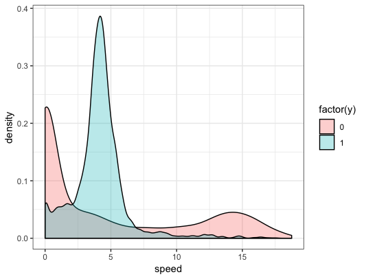
Animals might move at very low speeds when resting or sleeping (two possible non-foraging behaviors) and move at much higher speeds when migrating (another possible non-foraging behavior). The animals might move at sort of in-between speeds when foraging. In our data, which may or may not be representative of any actual animal, this pattern is apparent:
We might also imagine that depth (we’ll pretend these are marine predators) is a proxy for habitat and mayb the animals prefer to forage in certain types of habitat. Length will help control for heterogeneity (maybe different sized animals forage at different speeds or prefer different habitat), hour-of-day could capture potential preferences for foraging at night versus during the day, etc.
> summary(dat)
       X             foraging         utc_date                        lat             lon
 Min.   :     1   Min.   :0.0000   Min.   :2014-01-01 08:13:00   Min.   :32.81   Min.   :-126.0
 1st Qu.: 44932   1st Qu.:0.0000   1st Qu.:2014-04-30 22:41:02   1st Qu.:40.40   1st Qu.:-124.7
 Median : 89864   Median :0.0000   Median :2014-07-21 22:29:14   Median :44.60   Median :-124.3
 Mean   : 89864   Mean   :0.2794   Mean   :2014-07-08 04:59:03   Mean   :42.81   Mean   :-123.6
 3rd Qu.:134795   3rd Qu.:1.0000   3rd Qu.:2014-09-12 17:12:48   3rd Qu.:46.20   3rd Qu.:-123.9
 Max.   :179726   Max.   :1.0000   Max.   :2015-01-01 07:34:00   Max.   :48.75   Max.   :-117.3
   local_time                      depth               speed           bearing.rad
 Min.   :2014-01-01 00:13:00   Min.   :   0.0002   Min.   :    0.00   Min.   :0.0000
 1st Qu.:2014-04-30 15:41:02   1st Qu.:  59.1219   1st Qu.:    0.02   1st Qu.:0.1366
 Median :2014-07-21 15:29:14   Median : 181.8555   Median :    3.72   Median :2.6130
 Mean   :2014-07-07 21:59:03   Mean   : 282.4584   Mean   :    6.35   Mean   :2.5431
 3rd Qu.:2014-09-12 10:12:48   3rd Qu.: 464.5980   3rd Qu.:    7.65   3rd Qu.:4.4097
 Max.   :2014-12-31 23:34:00   Max.   :3077.3398   Max.   :45209.96   Max.   :6.2830
      hour           length            year          month
 Min.   : 0.00   Min.   : 31.00   Min.   :2014   Min.   : 1.000
 1st Qu.: 5.00   1st Qu.: 59.00   1st Qu.:2014   1st Qu.: 4.000
 Median :11.00   Median : 73.00   Median :2014   Median : 7.000
 Mean   :11.38   Mean   : 71.64   Mean   :2014   Mean   : 6.707
 3rd Qu.:17.00   3rd Qu.: 85.00   3rd Qu.:2014   3rd Qu.: 9.000
 Max.   :23.00   Max.   :129.00   Max.   :2014   Max.   :12.000
My goal here it to be able to predict whether an animal is foraging or not given it’s location and some other physical/environmental characteristics associated with its location. I’m going to fit 2 classes of models to my training data:
-
An Artificial Neural Network (ANN)
-
A Gradient Boosting Machine (GBM)
I’m going to use the functionality in caret to find the best ANN and the best GBM to predict the behavioral state of unlabeled observations.
The Models:
ANNs
It is important to try and understand the models and how they work. But there just isn’t enough space in a single blog post to really get into Stochastic Gradient Boosting and Artificial Neural Networks. Here’s the best I can do for some over simplified descriptions right now, along with several resources which I recommend for deeper reading.
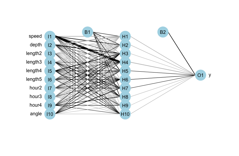
Artificial Neural Networks are kind of fun to take about because they’re easy to draw and therefore easy to explain on a conceptual level. Most of the hard stuff with ANNs happens behind the scenes. Here is an illustration of a sample neural network applied to my problem of predicting foraging versus non-foraging behavior of animals. It’s a network with 10 inputs, 1 hidden layer, and 10 nodes in the hidden layer.
The basic thing to understand about ANNs is that all of those lines connecting inputs to the various nodes in the hidden layer have a weight attached to them. Likewise, all those lines connecting the nodes of the hidden layer to the output layer have a weight attached to them. In the illustration above, B1 and B2 are bias layers (constant terms) that act sort of like intercept terms in a regression.
In a neural network, for a given set of hyper-parameters, an optimization algorithm finds the combination of weights that best predicts the outcome variable. There are potentially tons of hyper-parameters and modeling choices available for ANN models. Some of these are pretty standard across different Machine Learning models:
- what lose function to use
- what learning rate to use (the learning rate generally controls the tradeoff between getting stuck in local optima and taking forever to converge)
- what performance metric to use to decide on the ‘best’ model
Some hyper-parameters are kind of specific to ANNs:
- the number of nodes in the hidden layer
- the number of hidden layers to use
If you want a slightly more technical discussion of ANNs that still have lots of cool pictures:
GBM
Here is a really cool set of slides on Ensemble Trees and Gradient Boosting. The idea behind Ensemble Methods in Machine Learning is that by combining the predictions of serveral “weak” learners we can get a really strong model. When we talk Ensemble Methods applied to Tree-based models we are generally talking about a process where we:
- Grow a simple decision tree/regression tree/classification tree
- This tree gets some stuff right and gets some stuff wrong (has some error)
- Fit another tree to the error from 1.
- Rinse and repeat.
Gradient Boosting Trees is an iterative process. Each tree produces a prediction. The overall prediction is an aggregation of the predictions of each of the trees in the Ensemble.
Here is another summary of Gradient Boosted Trees that I really like.
Gradient Boost refers to the algorithm used to fit new trees: at each step in the process there is a loss function and we want to choose a tree that reduces the loss (to minimize overall loss we move according to the gradient of the loss function).
CARET
Using the caret library to train machine learning models, there are a few choices we need to make:
First, caret’s train() function includes a parameter for what model you want to train. Check out Chapter 6 here for the full list of models and libraries to choose from. These include, but are not limited to: Adaptive Boosting Classification Trees from the fastAdaboost library, Bayesian Adaptive Regression Trees from the bartMachine library, Neural Networks from the nnet library, Neural Networks from the neuralnet library, Generalized Partial Least Squares from gpls library…and literally about 600 more.
For my first class of model I’ve choosen ANNs but now I need to choose which library and method value I’m going to use. In this case, I’m choosing the nnet() method from the nnet library. The second model class that I’m experimenting with is Gradient Boosting Machines. Again, there are a couple of libraries in R that will do this flavor or learner…I’m going with Stochastic Gradient Boosting via the gbm() method in the gbm library.
Model Selection
# A proper CV experiment with ANNs

#--------------------------------------------------------------------
#create the training and testing data
index <- createDataPartition(df$y,p=0.8,list=F,times=1)
df.train <- df[index,] %>% mutate(y=as.factor(y))
levels(df.train$y) <- c('notforaging','foraging')
df.test <- df[-index,] %>% mutate(y=as.factor(y))
levels(df.test$y) <- c('notforaging','foraging')
#--------------------------------------------------------------------

#--------------------------------------------------------------------
# set up control parameters for the neural network
fitControl <- trainControl(method = "cv",
                           number = 5,
                           classProbs = TRUE,
                           summaryFunction = twoClassSummary)

nnetGrid <-  expand.grid(size = seq(from = 1, to = 10, by = 1),
                         decay = seq(from = 0.1, to = 0.5, by = 0.1))

# set up control parameters for the GBM
fitControl.GBM <- trainControl(method = "cv",
                               number = 5,
                               classProbs = TRUE,
                               summaryFunction = twoClassSummary)

# pre process the data....only the continuous variables
preProcValues <- preProcess(df.train, method = c("range"))
trainTransformed <- predict(preProcValues, df.train)
testTransformed <- predict(preProcValues, df.test)
#----------------------------------------------------------------------

#----------------------------------------------------------------------
# Train the models
t <- Sys.time()
nnetFit <- train(y ~ .,
                 data = trainTransformed,
                 method = "nnet",
                 metric = "ROC",
                 trControl = fitControl,
                 tuneGrid = nnetGrid,
                 verbose = FALSE)

# tree-based methods generally don't need input scaling
gbmFit <- train(y ~ .,
                data = df.train,
                method = "gbm",
                metric = "ROC",
                trControl = fitControl.GBM,
                verbose = FALSE)
Sys.time() - t
Time difference of 45.61796 mins
#-------------------------------------------------------------------------
The first thing one might notice is that even with a modest data set it takes a while to train the models. This is mostly due to the neural network: 5 fold cross-validation means each model is run 5 times. Since we have a grid of hyperparameters with 50 distinct combinations, we have 250 models that are evaluated here. Each of those 250 models is a different neural network and neural networks are generally pretty time costly to train (the backpropogation algorithm that is generally used to find optimal weights for the network nodes is pretty loop intensive).
Before moving on the prediction, I would like to highlight a few things here:
Preprocessing data before or during?
If I look at a few of the list objects returned by train() for the neural network I can confirm that no preprocessing took place within train() and that the training data are what I supplied.
> nnetFit$preProcess
NULL
> nnetFit$trainingData
# A tibble: 87,250 x 6
   .outcome    speed   depth length hour  angle
   <fct>       <dbl>   <dbl> <fct>  <fct> <dbl>
 1 notforaging     0 0.00663 3      3         0
 2 notforaging     0 0.00663 3      4         0
 3 notforaging     0 0.00663 3      4         0
 4 notforaging     0 0.00663 3      4         0
 5 notforaging     0 0.00663 3      4         0
 6 notforaging     0 0.00663 3      4         0
 7 notforaging     0 0.00663 3      4         0
 8 notforaging     0 0.00663 3      1         0
 9 notforaging     0 0.00663 3      1         0
10 notforaging     0 0.00663 3      1         0
An alternative to pre-processing data before supplying that data to train() would be to include a pre-processing option within the train() method. Here’s how that would look for my problem:
nnetFit2 <- train(y ~ .,
                 data = df.train,
                 method = "nnet",
                 preProcess=c('range'),
                 metric = "ROC",
                 trControl = fitControl,
                 tuneGrid = nnetGrid,
                 verbose = FALSE)
Here, I feed train() the original training data and include a pre-processing option inside the method call. Here’s the thing: when I pre-processed the data before passing it to train(), I used a normalization that transformed the continuous variables to the [0,1] interval. This was done using:
preProcValues <- preProcess(df.train, method = c("range"))
trainTransformed <- predict(preProcValues, df.train)

> preProcValues
Created from 87250 samples and 6 variables

Pre-processing:
  - ignored (3)
  - re-scaling to [0, 1] (3)
This transformation basically left my 3 factor-type variables alone and transformed my 3 continuous variables.
When I include the pre-processing inside of my call to train(), I don’t really know what’s going on but I don’t love it. It looks like all of my variables are being transformed. Maybe this doesn’t matter much, but I don’t like rescaling categorical variables…it doesn’t make sense to me.
> nnetFit2$preProcess
Created from 87250 samples and 10 variables

Pre-processing:
  - ignored (0)
  - re-scaling to [0, 1] (10)
One-hot Encoding
Read more about One-Hot Encoding Here.
When I first starting running neural network models using train() I was pretty confused about why I was feeding it 5 input variables and it was coming back to me with 10 input models. At first, I thought the train() function was doing it’s own feature selection and maybe adding interaction terms and testing them on it’s own.
While it seems that, caret::train() does have feature selection methods, this is not what was happening in my case. In my case, since lenght and hour-of-day are categorical factor variables, the nnet() method that is called by train converts the categorical variables to a set of dummy variables (one-hot encoding). Since length has 5 levels, the first one is dropped and 4 dummy variables are created. Hour-of-day has 4 levels so the first one is dropped and we have dummy variables for hour2, hour3, and hour4.
> nnetFit$finalModel
a 10-10-1 network with 121 weights
inputs: speed depth length2 length3 length4 length5 hour2 hour3 hour4 angle
output(s): .outcome
options were - entropy fitting  decay=0.1
>
Prediction
Now we have two model objects nnetFit and gbmFit that contain the best ANN and best GBM models given the methods and hyperparameters that we searched over. To see how these optimal models perform on the testing data we can use the predict() method:
#-------------------------------------------------------------------------
# make predictions
NNpredictions <- predict(nnetFit,testTransformed)
GBMpredictions <- predict(gbmFit,df.test)

> head(NNpredictions)
[1] notforaging notforaging notforaging notforaging notforaging foraging
Levels: notforaging foraging
> head(GBMpredictions)
[1] notforaging notforaging notforaging notforaging notforaging foraging
Levels: notforaging foraging
#------------------------------------------------------------------------
A popular way of evaluating predictive performance in the ML community is using the confusion matrix. The confusion matrix could be generated by hand without too much trouble since the object NNpredictions is a just a vector of predictions for the test data….but caret has a confusionmatrix() method which can also do the work for us:
confmat <- confusionMatrix(NNpredictions,testTransformed$y)
GBMmat <- confusionMatrix(GBMpredictions,df.test$y)

> confmat$table
             Reference
Prediction    notforaging foraging
  notforaging       15232     1976
  foraging           1655     2949

> GBMmat$table
             Reference
Prediction    notforaging foraging
  notforaging       15627     1236
  foraging           1260     3689
With ML models it’s also popular to evalute performace using an F1 Score which is a weighted average of a model’s precision and recall. We calculate F1 for our two models by hand as follows:
#f1 score for the ANN
p <- confmat$table[2,2]/(confmat$table[2,2] + confmat$table[2,1])
r <- confmat$table[2,2]/(confmat$table[2,2] + confmat$table[1,2])
(2*p*r)/(p+r)
[1] 0.6189527

#f1 score for the GBM
p <- GBMmat$table[2,2]/(GBMmat$table[2,2] + GBMmat$table[2,1])
r <- GBMmat$table[2,2]/(GBMmat$table[2,2] + GBMmat$table[1,2])
(2*p*r)/(p+r)
[1] 0.7472149
Recap
Ok, there’s a lot of stuff in this post. The main thing I want to stress is that caret has a method called train() that works with an almost endless array of machine learning models. I find the syntax and functionality really appealing. For a final example of why, consider this:
Suppose I want to fit an Artifical Neural Network model to some data to make predictions using the nnet library. Per the documentation, the nnet() function fits an ANN with a single hidden layer. The main hyper-parameters that the user controls are:
- size = the number of nodes in the hidden layer of the network (just to be clear, if you want to also control the number of hidden layers, you need to use a different ANN library like neuralnet)
- decay = a regularization parameter to avoid overfitting
Suppose I want to do a 5 fold cross-validation using nnet() to determine the best network
# suppose I have training data called train
# suppose I have testing data called test
# suppose the target variable is called y
# suppose the input variables are x1, x2, x3

netsize <- c(1:10)
netdecay <- seq(from = 0.1, to=0.5, by=0.1)
mod <- list()

for(i in netsize){
 for(j in netdecay){
 tmpmod <- list()
   for(k in unique(train$fold)){
    NN <- nnet(y~x1+x2+x3,train,size=i,decay=j,lineout=F)
    test$pred <- predict(NN,test,type='class')
    p <- nrow(test[test$y=='foraging' & test$pred=='foraging'])/(nrow(test[test$y=='foraging' & test$pred=='foraging',])+
                 nrow(test[test$y=='notforaging' & test$pred=='foraging']))
    r <- nrow(test[test$y=='foraging' & test$pred=='foraging'])/(nrow(test[test$y=='foraging' & test$pred=='foraging',])+
                 nrow(test[test$y=='foraging' & test$pred=='notforaging']))
    f1 <- (2*p*r)/(p+r)
    tmpmod[[k]] <- f1
    }
   mod[[i,j]] <- mean(unlist(tmpmod))

 }
 }
Basically, I can manually loop through a bunch of hyperparameters, do a 5 fold CV on each unique combination, save all the performace metrics, then find the best one. Or I can do:
#--------------------------------------------------------------------
# set up control parameters for the neural network
fitControl <- trainControl(method = "cv",
                           number = 5,
                           classProbs = TRUE,
                           summaryFunction = twoClassSummary)

nnetGrid <-  expand.grid(size = seq(from = 1, to = 10, by = 1),
                         decay = seq(from = 0.1, to = 0.5, by = 0.1))

# pre process the data....only the continuous variables
preProcValues <- preProcess(df.train, method = c("range"))
trainTransformed <- predict(preProcValues, df.train)
testTransformed <- predict(preProcValues, df.test)

nnetFit <- train(y ~ .,
                 data = trainTransformed,
                 method = "nnet",
                 preProcess=c('range'),
                 metric = "ROC",
                 trControl = fitControl,
                 tuneGrid = nnetGrid,
                 verbose = FALSE)
It may or may not be fewer lines of code…but it’s more readable and more elegant in my opinion.