
A Fun State Space Simulation Exercise
In this earlier post I tried to provide some helpful nuggets regarding the use of R’s KFAS package for modeling monthly seasonal data using a state space framework. I was going to add a little simulation experiment I cooked up just to further my understanding of how KFAS and state space models behave…but that post got a little long so I decided to include the simulation as a separate, companion post.
Play Along Here
Outline
In this post I used monthly data on number of commercial fishing trips taken off a section of the U.S. West Coast (to maintain confidentiality of the data I cannot tell you which section) and fit a structural time series model using the state space framework.
My goal here was to examine whether seasonality was constant over time (in the sense that fishing effort tend to be higher during some months and lower during other months and that these highs and lows occur in roughly the same months every year). To address this question I estimated two different models:
-
A state space model which was pretty flexible in the sense that it allows the monthly seasonal effect to differ each year (time varying seasonal effects).
-
A seasonal dummy variable regression with a structural break. Conceptually, this model is a bit more rigid. If seasonal effects were reasonably consistent over some subsample of the data then change notably at a certain point in time to a different seasonal pattern this model should perform pretty well. However, if seasonal effects are changing in small ways consistently through time, we would expect this model to perform poorly.
In the real world example the state space model fit pretty well…I suspected this was because the pattern of seasonality appeared to be a slow evolution from a July peak to an August peak. Since I appeared to have a good example in hand of where the flexibility of a state space model outperforms the rigidity of a deterministic seasonal model represented by the seasonal dummy variable model, I thought it would be cool to try and conceptualize the opposite….that is, a system where the seasonal dummy variable regression with a structural break outperforms the state space model.
Here is what I came up with:
-
Simulate a time-series of monthly data where the monthly means are fixed for \(t=1,...k\) and fixed at different levels for \(t=k+1,...T\).
-
Fit the same seasonal state space model as we used for the fishing data.
-
Fit a monthly dummy variable regression model with a structural break at \(t=k\)
-
Compare.
Experiment
Step 1: Simulate the data
#----------------------------------------------------------------
#simulate data that is seasonal but with seasonality that shifts at some point
means <- c(10,20,30,40,50,60,70,40,30,20,20,10)
means2 <- c(70,60,50,40,30,20,10,20,30,40,60,70)

df <- rbind(
  data.frame(trips.s=rnorm(10,means[1],5),year=c(1995:2004),month=1),
  data.frame(trips.s= rnorm(10,means[2],5),year=c(1995:2004),month=2),
  data.frame(trips.s=rnorm(10,means[3],5),year=c(1995:2004),month=3),
  data.frame(trips.s=rnorm(10,means[4],5),year=c(1995:2004),month=4),
  data.frame(trips.s=rnorm(10,means[5],5),year=c(1995:2004),month=5),
  data.frame(trips.s=rnorm(10,means[6],5),year=c(1995:2004),month=6),
  data.frame(trips.s=rnorm(10,means[7],5),year=c(1995:2004),month=7),
  data.frame(trips.s=rnorm(10,means[8],5),year=c(1995:2004),month=8),
  data.frame(trips.s=rnorm(10,means[9],5),year=c(1995:2004),month=9),
  data.frame(trips.s=rnorm(10,means[10],5),year=c(1995:2004),month=10),
  data.frame(trips.s=rnorm(10,means[11],5),year=c(1995:2004),month=11),
  data.frame(trips.s=rnorm(10,means[12],5),year=c(1995:2004),month=12)
)

df <- tbl_df(df) %>% mutate(date=as.Date(paste(year,"-",month,"-","01",sep=""),format="%Y-%m-%d")) %>%
  arrange(year,month) %>% mutate(july=ifelse(month==7,1,0))

df.post <- rbind(
  data.frame(trips.s=rnorm(5,means2[1],5),year=c(2005:2009),month=1),
  data.frame(trips.s= rnorm(5,means2[2],5),year=c(2005:2009),month=2),
  data.frame(trips.s=rnorm(5,means2[3],5),year=c(2005:2009),month=3),
  data.frame(trips.s=rnorm(5,means2[4],5),year=c(2005:2009),month=4),
  data.frame(trips.s=rnorm(5,means2[5],5),year=c(2005:2009),month=5),
  data.frame(trips.s=rnorm(5,means2[6],5),year=c(2005:2009),month=6),
  data.frame(trips.s=rnorm(5,means2[7],5),year=c(2005:2009),month=7),
  data.frame(trips.s=rnorm(5,means2[8],5),year=c(2005:2009),month=8),
  data.frame(trips.s=rnorm(5,means2[9],5),year=c(2005:2009),month=9),
  data.frame(trips.s=rnorm(5,means2[10],5),year=c(2005:2009),month=10),
  data.frame(trips.s=rnorm(5,means2[11],5),year=c(2005:2009),month=11),
  data.frame(trips.s=rnorm(5,means2[12],5),year=c(2005:2009),month=12)
)

df.post <- tbl_df(df.post) %>% mutate(date=as.Date(paste(year,"-",month,"-","01",sep=""),format="%Y-%m-%d")) %>%
  arrange(year,month) %>% mutate(july=ifelse(month==7,1,0))

#----------------------------------------------------------------
# slightly different simulation
error <- rnorm(120,0,5)
chow2.df <- tbl_df(data.frame(year=c(rep(1995,12),rep(1996,12),rep(1997,12),rep(1998,12),
                                     rep(1999,12),rep(2000,12),rep(2001,12),
                                     rep(2002,12),rep(2003,12),rep(2004,12)),
                              month=rep(1:12,10),
                              int=11.206,error=error)) %>%
  mutate(
    feb=ifelse(month==2,7.8,0),
    march=ifelse(month==3,17.47,0),
    april=ifelse(month==4,30.5,0),
    may=ifelse(month==5,38.2,0),
    june=ifelse(month==6,49.4,0),
    july=ifelse(month==7,59.3,0),
    aug=ifelse(month==8,26.2,0),
    sept=ifelse(month==9,19.2,0),
    oct=ifelse(month==10,11.8,0),
    nov=ifelse(month==11,7.4,0),
    dec=ifelse(month==12,0.8,0),
    trips.s=int+feb+march+april+may+june+july+aug+sept+oct+nov+dec+error,
    date=as.Date(paste(year,"-",month,"-","01",sep=""),format="%Y-%m-%d")) %>%
  arrange(year,month)
error <- rnorm(72,0,5)
chow2.df2 <- tbl_df(data.frame(year=c(rep(2005,12),rep(2006,12),rep(2007,12),rep(2008,12),
                                      rep(2009,12),rep(2010,12)),
                               month=rep(1:12,6),
                               int=69.6,error=error)) %>%
  mutate(
    feb=ifelse(month==2,-10.6,0),
    march=ifelse(month==3,-16.5,0),
    april=ifelse(month==4,-27.4,0),
    may=ifelse(month==5,-37.8,0),
    june=ifelse(month==6,-50.5,0),
    july=ifelse(month==7,-61.6,0),
    aug=ifelse(month==8,-50.35,0),
    sept=ifelse(month==9,-37.11,0),
    oct=ifelse(month==10,-26.5,0),
    nov=ifelse(month==11,-8.5,0),
    dec=ifelse(month==12,-3.1,0),
    trips.s=int+feb+march+april+may+june+july+aug+sept+oct+nov+dec+error,
    date=as.Date(paste(year,"-",month,"-","01",sep=""),format="%Y-%m-%d")) %>%
  arrange(year,month)

chow2.df <- chow2.df %>% select(trips.s,year,month,date) %>% mutate(july=ifelse(month==7,1,0))
chow2.df2 <- chow2.df2 %>% select(trips.s,year,month,date) %>% mutate(july=ifelse(month==7,1,0))

#---------------------------------------------------------------

#combine the two data frames
ss.data <- rbind(df,df.post)
#ss.data <- rbind(chow2.df,chow2.df2)

#give the data a trend
trend <- 2
c <- c(200,rep(0,length(ss.data$trips.s)-1))
for(i in 2:length(c)){
  c[i]<- c[i-1] + trend + rnorm(1,0,1)
}

ss.data$c <- c
ss.data$trips <- ss.data$c + ss.data$trips.s
ss.data$t <- seq(1:nrow(ss.data))
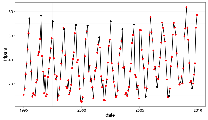
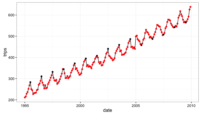
What I’ve done here is simulated a monthly seasonal process with a little bit of noise that, from 1995 to 2004 peaks in July, then, from 2005 to 2009 peaks in December-January with a trough in July. So the system abruptly switches from high summer values and low winter values to high winter values and low summer values.
In the simulated data the column trips follows the seasonal dynamics but also has a consistent positive upward trend. The series trips.s is not influenced by the persistent trend.
Step 2: Fit the state space models
We simulated 2 data series, trips and trips.s. To model these two series we will specify two different state space models. Both models with introduce seasonal effects through monthly dummy variables but one model (tripsModel_trend) will also have a local time varying level…the model tripsModel does not have this SSMtrend component. Both models allow time varying seasonal effects that are primarily captured through the process error variance, Q.
#-----------------------------------------------------------------------------------
#specify a state-space model with seasonals only
dates <- ss.data$date
trips <- xts(ss.data$trips.s,order.by=dates)
trips.trend <- xts(ss.data$trips, order.by=dates)

tripsModel<-SSModel(trips ~ SSMseasonal(period=12, sea.type="dummy", Q = NA), H = NA)

#state space model with local level and seasonals
tripsModel_trend<-SSModel(trips ~ SSMtrend(degree = 1, Q=list(matrix(NA))) +
                      SSMseasonal(period=12, sea.type="dummy", Q = NA), H = NA)

#---------------------------------------------------------------------------------

#--------------------------------------------------------------------------------
#Get the likelihood maximizing parameter values for the model
tripsFit<-fitSSM(tripsModel,inits=c(0.05, 0.001),method='BFGS')$model
tripsFit_trend<-fitSSM(tripsModel,inits=c(0.1,0.05, 0.001),method='BFGS')$model

#Get the smoothed estimates of the state values
tripsSmooth <- KFS(tripsFit,smooth= c('state', 'mean','disturbance'))
tripsSmooth_trend <- KFS(tripsFit,smooth= c('state', 'mean','disturbance'))

#Get smoothed estimates of the level
#tripsLevel <-signal(tripsSmooth, states = 'level')
#tripsLevel$signal <- xts(tripsLevel$signal, order.by = dates)
#autoplot(cbind(trips, tripsLevel$signal),facets = FALSE)
#-----------------------------------------------------------------------------

#---------------------------------------------------------------------------
#extract the seasonal
trips.sea <- as.numeric(tripsSmooth$alphahat[,2])
plot.df <- data.frame(date=dates,seasonal=trips.sea)

trips.sea_trend<- as.numeric(tripsSmooth_trend$alphahat[,2])

#add a reference point to the seasonal data frame
plot.df <- plot.df %>% mutate(month=month(date),july=ifelse(month==7,1,0))


#-----------------------------------------------------------------------------
Step 3: fit the seasonal dummy variable models
Here we fit 2 distinct seasonal dummy variable regression models in order to do an apples-to-apples comparison with our state space model.
The first model is not impacted by the persistent trend and we use the series trips.s on the left-hand side and include on the right-hand side only the monthly dummy variables. We estimate the separately in each of two time periods to account for the structural break.
The second model is impacted by the persistent trend and uses the series trips on the left-hand side and includes as regressors the monthly dummy variables as well as a time trend. This model is also estimated separately for two sub-samples of the data to capture the structural break in 2004/2005.
#===========================================================
#Compare our state-space model with a dummy variable regression
# with structural break:

chow.df <- ss.data %>%
  mutate(jan=ifelse(month==1,1,0),
         feb=ifelse(month==2,1,0),
         march=ifelse(month==3,1,0),
         april=ifelse(month==4,1,0),
         may=ifelse(month==5,1,0),
         june=ifelse(month==6,1,0),
         july=ifelse(month==7,1,0),
         aug=ifelse(month==8,1,0),
         sept=ifelse(month==9,1,0),
         oct=ifelse(month==10,1,0),
         nov=ifelse(month==11,1,0),
         dec=ifelse(month==12,1,0))


model.pre <- lm(trips.s~feb+march+april+may+june+july+aug+
                  sept+oct+nov+dec,data=subset(chow.df,year<=2004))
model.pre.trend <- lm(trips~feb+march+april+may+june+july+aug+
                  sept+oct+nov+dec+t,data=subset(chow.df,year<=2004))

model.post <- lm(trips.s~feb+march+april+may+june+july+aug+
                   sept+oct+nov+dec,data=subset(chow.df,year>2004))

model.post.trend <- lm(trips~feb+march+april+may+june+july+aug+
                   sept+oct+nov+dec+t,data=subset(chow.df,year>2004))


yhat <- rbind(
  data.frame(date=chow.df$date[chow.df$year<=2004],
             that=predict(model.pre,newdata=chow.df[chow.df$year<=2004,])),
  data.frame(date=chow.df$date[chow.df$year>2004],
             that=predict(model.post,newdata=chow.df[chow.df$year>2004,]))
)

yhat_trend <- rbind(
  data.frame(date=chow.df$date[chow.df$year<=2004],
             that=predict(model.pre.trend,newdata=chow.df[chow.df$year<=2004,])),
  data.frame(date=chow.df$date[chow.df$year>2004],
             that=predict(model.post.trend,newdata=chow.df[chow.df$year>2004,]))
)


yhat$y <- as.numeric(trips)
yhat$model <- 'Seasonal Dummy'

yhat_trend$y <- as.numeric(trips.trend)
yhat_trend$model <- 'Seasonal Dummy w/trend'
Step 4: Model Comparison
Here we compare:
-
The seasonal state space model with no SSMtrend component (fit to the data with no persistent trend) to the monthly dummy variable regression (also fit to the data with no persistent trend)…and
-
The seasonal state space model with an SSMtrend component (fit to the simulated data with persistent trend) to the monthly dummy variable regression with a time trend (also fit to the data with the persistent trend):
# the KFAS model
kfas.pred <- data.frame(date=dates,that=fitted(tripsSmooth),y=as.numeric(trips),model='KFAS')
kfas.pred_trend <- data.frame(date=dates,that=fitted(tripsSmooth_trend),y=as.numeric(trips.trend),model='KFAS trend')

#combine the two
model.comp <- rbind(yhat,yhat_trend,kfas.pred,kfas.pred_trend)

model.comp$eps <- model.comp$y-model.comp$that

tbl_df(model.comp) %>% mutate(abs.error=abs(eps)) %>% group_by(model) %>%
  summarise(mean(abs.error,na.rm=T))

  # A tibble: 4 × 2
                   model `mean(abs.error, na.rm = T)`
                   <chr>                        <dbl>
1                   KFAS                  6.490529250
2             KFAS trend                  0.002371808
3         Seasonal Dummy                  3.470531813
4 Seasonal Dummy w/trend                  4.212804855
>
Discussion:
A few observations:
The state space model with seasonals only “oversmooths”
Smoothing is generally pretty awesome because we have lots of super flexible techniques that can allow us, mathematically/empirically at least, to fit a line really close to an arbitrary set of data points no matter how squiggly they are…people concerned with generating insight from data usually try to avoid doing this and sometimes call it, “chasing noise.”
In this case, we have an abrupt shift in the system at a discrete point in time. The seasonal only state space model estimates a constant intercept term roughly around the unconditional mean of the data. The seasonal impact is then estimated as the monthly variation around the unconditional mean.
Let’s take a pictoral look at what is going on focusing on the shift from July peak 1995-2004 to July trough 2005 - 2009:
Initially, the July values are consistently around 70. After 2004 they shift and are consistently around 20.
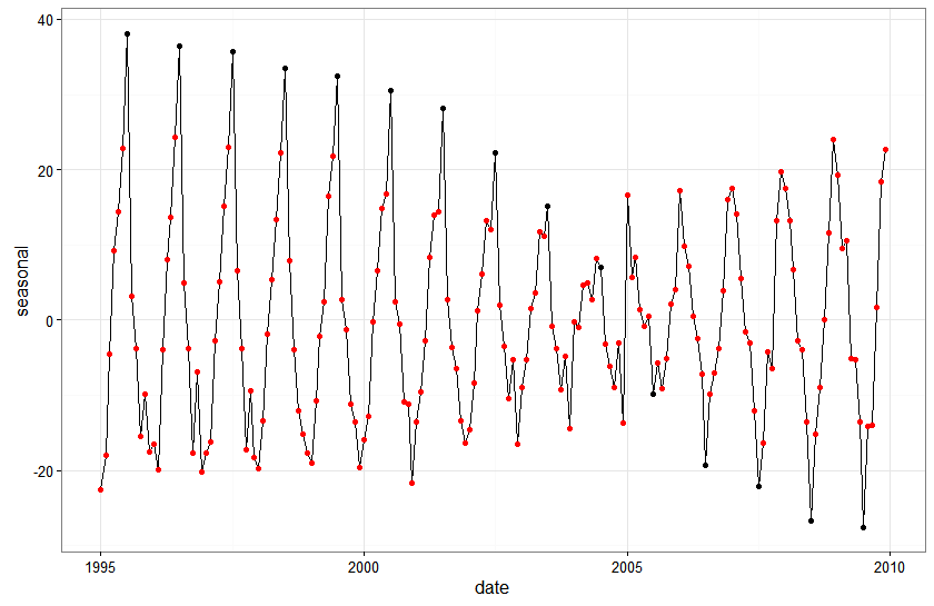
If we look at the seasonal estimates from the state space model we can get some intuition for how the model is treating this shift. Rather than introducing a discrete shift between 2004 and 2005, the model is smoothing out the transition from high July values to low July values by gradually decreasing the seasonal effect associated with July observations. This makes sense from a structural modeling perspective in that we have specified a model where the seasonal component is a random walk with drift…so the seasonal impact in each period should be a function of the estimated impact for the same month last year plus some noise.
Basically, and this may be a gross over simplification but….the data are saying that the July series starts at 70 and ends at 10. The model is saying that the best way to get there is to shave a little off the estimated seasonal effect every year.
#like we did in our previous post we extract the seasonal from the KFAS object by getting the 'alphahat' element of that object:

ggplot(plot.df,aes(x=date,y=seasonal)) + geom_line() + geom_point(aes(color=factor(july))) +
  scale_color_manual(values=c('red','black')) +
  theme_bw() +
  theme(legend.position="none")
In contrast, dummy variable regression with structural break fits better because it doesn’t assume a slow transition from high July values to low July values. The seasonal effects are fixed across the two distinct data subsamples.
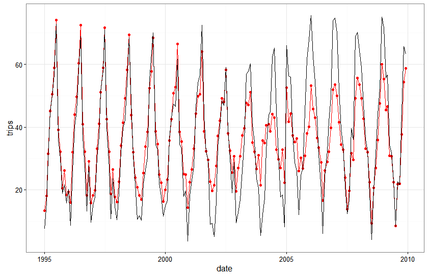
Here is a plot of the fitted values against actual values for the seasonal state space model with no local level…with observed values in black and fitted values in red:
ggplot(subset(model.comp,model%in%c('KFAS')),aes(x=date,y=that)) + geom_line(color='red')+ geom_point(color='red') +
  geom_line(aes(x=date,y=y),color="black") + theme_bw()
And here is the same plot for the seasonal dummy variable regression with the correct structural break:
ggplot(subset(model.comp,model%in%c('Seasonal Dummy')),aes(x=date,y=that)) + geom_line(color='red')+ geom_point(color='red') +
  geom_line(aes(x=date,y=y),color="black") + theme_bw()
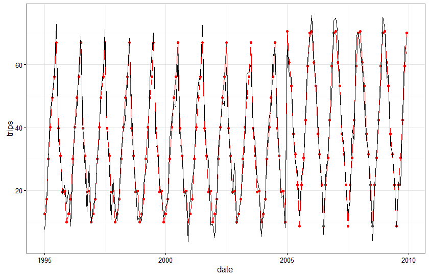
The seasonal state space model actually looks really good…everywhere except right around the area of the structural break. What’s also pretty cool to note is that the fit of the state space model gets better every year following the break…the structural break messes it up for a year or two but the flexible dynamics in the model adjust to the break pretty quickly.
The seasonal state space model with local level fits great….without actually capturing the right seasonal dynamics
The local level model with seasonal factors has a time varying level that is really good at picking up variation and hence creating a really good fit to the data. However, it swallows up a lot of the variation that probably should get assigned to the seasonal effect.
Let’s have a look. Here I’m printing out side-by-side: i) the smoothed estimate of the level at each time period, ii) the smoothed estimate of the seasonal impact, iii) the actual trending level from the data generating process, iv) the actual seasonal effect from the data generating process, and v) the observed number of trips:
z <- data.frame(dates=dates,ssm_int=tripsSmooth_trend$alphahat[,1],sea=tripsSmooth_trend$alphahat[,2],trend=ss.data$c,y.sea=ss.data$trips.s,y=ss.data$trips)

print.data.frame(z[1:24,])

print.data.frame(z[100:120,])
Even though the fit of the model to the data is really good, we note that, in almost every period, the smoothed estimate of the seasonal effects is pretty far off from the underlying seasonal used to build the data…
WARNING: I haven’t thought super hard about this issue yet. It could be that I’m interpreting the model and results incorrectly. It could be that I set up an simulation with really poor identifiability. At the moment I don’t really know what/how much to make of this issue of good fit with the ‘wrong’ decomposition.’
Could we find the ‘right’ break if we didn’t know it was there a priori?
It’s somewhat trivial in this exercise to observe that the seasonal dummy variable model with a structural break in 2004/2005 has lower mean absolute in-sample prediction error. After all, the simulated system has pretty predictable seasonality with relatively low error variance and we specified the structural break correctly because we knew where it was.
What if we had to test for the location of the structural break?
break.test <- function(yr){
sb.df <- chow.df %>% mutate(sbreak=ifelse(year==yr,1,0))

  sb <- lm(trips.s~feb+march+april+may+june+july+aug+sept+oct+nov+dec+
           feb*sbreak+march*sbreak+
           april*sbreak+may*sbreak+june*sbreak+july*sbreak+
           aug*sbreak+sept*sbreak+sept*sbreak+oct*sbreak+
           nov*sbreak+dec*sbreak,data=sb.df)
return(extractAIC(sb))
}
> lapply(c(2003:2008),break.test)
[[1]]
[1]   24.00 1085.09

[[2]]
[1]   24.000 1082.782

[[3]]
[1]   24.000 1064.262

[[4]]
[1]   24.0 1064.4

[[5]]
[1]   24.00 1061.04

[[6]]
[1]   24.000 1065.382
Kinda looks like if we didn’t know where the structural break was, even with these data that shift really abruptly and without too much noise, we could reach some pretty ambiguous conclusions about where the break occurs.
DISCLAIMER: AIC on the dummy variable model with interaction term is probably not the most rigorous way to test and date structural breaks in a seasonal model. For starters it’s probably better to use a Bai and Perron (2002) type test for testing and dating multiple potential change points.
Final Thoughts
I’m sorry I don’t have more concrete guidance for you on dynamic seasonal issues. I’m still trying to get a good understanding of them myself. This post was more about showing you a couple of really simple things I did in order to try and draw some pictures that would help me understand the models and processes a bit more.
If there is anything useful to take away from this exercise it might be this:
-
State space models are really flexible. You can stack level, seasonal, cyclic, and other terms together pretty easily…and these components can all have their own dynamics…or they can have coupled dynamics. This flexibility is really cool….like when it gives you a really nice fit or let’s you make really good one-step-ahead predictions of a time-series process.
-
This flexibility can also be costly. We showed that a state space model with a local level was capable of providing a really awesome fit to a seasonal time-series with a trending level…but that same model actually produced rather poor insight into the magnitude of the seasonal effects.