
State Space Models with Seasonal Data
A little while back I wrote a few posts on time-series methods for seasonal data.
While I mentioned state space models as an option for modeling seasonal data, I didn’t really provide much meat there. In this post I’m going to give a few examples applying state space models (using the ‘KFAS’ package in R) to seasonal data.
Much has been written about state-space modeling and most of it by people with substantially more expertise than I have. I’m not going to try and compete with the experts on statistical depth….my focus here will be on providing a few reproducible examples you can use to get the feel of how state-space models with the KFAS package behave.
For more depth on state space models I recommend (in order):
and if you’re looking for a nice code-based tutorial on R’s KFAS, state space models, and time-series in general, my colleague, Roy Mendelsohnn, has pretty easy to follow R Notebook available online:
If you want to follow along I have the code for this post reasonably well annotated in my cool-time-series-stuff GitHub repo, in the file: “ssm.R”.
Quick State-Space Introduction
As an economist I favor the basic illustration of state space models in the context of time-varying regression parameters. Consider the linear model $y=Z’\alpha$, where $\alpha$ is a vector of coefficients, $Z$ a data matrix, and $y$ a vector of dependent variables.
If we want to allow the marginal impact of the exogenous variables to evolve over time we might write the system as:
MODEL 1:
\[y_{t}=Z_{t} \alpha_{t} + \epsilon_{t}\] \[\alpha_{t+1}=T_{t}\alpha_{t} + R_{t}\eta_{t}\]The state-space framework is attractive to many researchers because it results in a pretty straightforward likelihood function which can be estimated using familiar methods.
Filtering and Smoothing
Filtering
I was trying to avoid getting too deep into this but I think it’s important for some stuff I want to do later in the post so here goes:
The garden variety Gaussian state space model can be obtained by adding a little structure to the set up above. Namely,
MODEL 2:
\(y_{t}=Z_{t} \alpha_{t} + \epsilon_{t}\), with \(\epsilon_{t} \sim N(0,H_{t})\)
\(\alpha_{t+1}=T_{t}\alpha_{t} + R_{t}\eta_{t}\), with \(\eta_{t} \sim N(0,Q_{t})\), and
\[\alpha_{1} \sim N(a_{t},P_{1})\]The Kalman Filter is the dominant estimation strategy for most state-space models. The Kalman Filter provides information on the unknown latent state (\(\alpha\)) by iteratively calculating a one-step ahead expected value and covariance matrix for the state vector:
\[a_{t+1}=E(\alpha_{t+1}|y_{t},...,y_{1})\] \[v_{t} = y_{t} - Z_{t}\alpha_{t}\] \[P_{t+1}=Var(\alpha_{t+1}|y_{t},...y_{1})\] \[F_{t}=Var(v_{t})=Z_{t}P_{t}^{T}+H_{t}\]Parameter Estimation
Given an initial values \(a_{1},P_{1}\) and variance parameters \(H_{t},Q_{t}\) a well-known logliklihood function can be derived for the basic Gaussian State Space model:
\[log L=-\frac{np}{2}log 2\pi - \frac{1}{2} \sum_{t=1}^{n}(log |F_{t}|+v_{t}'F_{t}^{-1}v_{t})\]Smoothing
The Kalman Filter helps us solve the likelihood maximization problem (note tha the liklihood function gets solved iteratively since, acording to the Kalman Filter, \(F_{t}\) relies on information up to time \(t-1\), \([y_{1},...y_{t-1}]\)) to obtain optimal estimates for the process and measurement error variances…which is cool…but I am generally more interested in the smoothed estimates of the state vector:
\[\hat{\alpha_{t}}=E(\alpha_{t}|y_{1},...y_{n})\] \[V_{t}=Var(\alpha_{t}|y_{1},...,y_{n})\]In a seasonal model, the smoothed state estimates give us the optimal ex-post estimate of the marginal seasonal impact in each time period…using all available data.
A Seasonal State Space Model in R
Here we will use some non-confidential data I have on the number of fishing trips taken in the West Coast Groundfish Fishery over time. The data are monthly from 1994 - 2014 and the variable ‘trips’ is a count of the total number of fishing trips taken in that month. The practical background here is that there have been multiple policy changes over time and I am interested in whether any of these regulatory events have altered the seasonal pattern of fishing activity.
library(Quandl)
library(KFAS)
library(dplyr)
library(ggplot2)
library(lubridate)
library("ggfortify")
library(xts)

#Read in the groundfish effort data------------------------------
df.monthly <- readRDS('data/gf_monthly.RDA')
#----------------------------------------------------------------
Next, we’ll do some simple processing and plot the series. I’m cheating a bit here but I know there is a pretty consistent summer peak in these data….In the plot below I mark the ‘July’ observations with a black dot and other months are red.
#create a univariate ts object---------------------------------
trips <- df.monthly$ntrips
#--------------------------------------------------------------

#do some other convenience operations---------------------------
df.monthly$date <- as.Date(paste(df.monthly$year,"-",df.monthly$month,"-","01",sep=""),format="%Y-%m-%d")
dates <- df.monthly$date
trips <- xts(trips,order.by=dates)

df.monthly <- df.monthly %>% mutate(july=ifelse(month==7,1,0))
#-----------------------------------------------------------------

#-------------------------------------------------------------------
# a few quick illustative plots
ggplot(df.monthly,aes(x=date,y=ntrips)) + geom_line() +
  geom_point(aes(color=factor(july))) +
  scale_color_manual(values=c('red','black')) +
  theme_bw() +
  theme(legend.position='none')
#---------------------------------------------------------------------
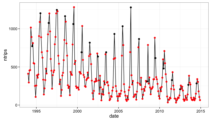
Note that from 1994 to 2010 we get a consistent seasonal peak in July (with some noise as, in some years the peak is June and others it is August). Also note that from 2011 to 2014 we get a very consistent August peak. This is important to me because in Jan. 2011 the West Coast Groundfish Fishery transitioned to a new management model. An open question, that part of my research will hopefully inform, is whether or not this management transition altred seasonality in the fishery.
Next, I’m going to fit a state-space model to these seasonal data. First, let’s get a little more specific about our seasonal state-space model:
Seasonal State-Space Model in R and ‘KFAS’
The first thing to note here is that the basic presentation of the standard structural time-series decomposition is to express a time-series of observations $y_{t}$ as a function of a level, seasonal, and cyclical component:
MODEL 3:
\[y_{t}=\mu_{t} + \gamma_{t} + c_{t}\]where $\mu_{t}$ is the level, $\gamma_{t}$ is the seasonal, and $c_{t}$ is the cyclical component.
Consider the familiar seasonal dummy variable regression model with monthly observations:
\[y_{t}=\alpha + \sum_{i=1}^{11}D_{i}\beta_{i}\]where $D_{i}$ equal 1 if observation $t$ is in month $i$ and 0 otherwise.
If we were to re-write the $\alpha$ term from the original state-space representation as,
\[\alpha_{t} = [\mu_{t},\gamma_{1,t},\gamma_{2,t},...\gamma_{11,t}]\]then it’s pretty easy to see how the basic structural time-series model can be expressed as a state-space model.
SSMtrend and SSMseasonal in KFAS
A structural time series model where the series is decomposed into a level/trend component and a seasonal component can be formally written in Gaussian state space form as:
MODEL 4:
\(y_{t} = \mu_{t} + \gamma_{t} + \epsilon_{t}\), where \(\epsilon_{t} \sim N(0,H_{t})\)
\(\mu_{t+1} = \mu_{t} + v_{t} + \eta_{t}\), where \(\eta_{t} \sim N(0,Q_{level,t}\)
\(v_{t+1} = v_{t} + \zeta_{t}\), where \(\zeta_{t} \sim N(0,Q_{slope,t})\)
\(\gamma_{t+1} = -\sum_{j=1}^{s-1}\gamma_{t+1-j} + w_{t}\), where \(w_{t} \sim N(0,Q_{seasonal,t})\)
In the ‘KFAS’ package in R, one can build a structural time series models additively using the function:
- SSMtrend(), and
- SSMseasonal()
Note that MODEL 4 above consists of a time varying level and a time-varying slope (\(\mu_{t+1}=\mu_{t} + v_{t}\))). If we wanted to build this model in KFAS we could do it additively like so
mymodel <- SSModel(y ~ SSMtrend(degree = 2, Q = list(matrix(1), matrix(0.5))) +
                       SSMseasonal(period=12, sea.type="dummy", Q = 0.5), H = 0.5)
An interesting thing to note here is that KFAS interprets ‘NA’ values as estimable parameters…so if we wanted to estimate the variance parameters rather than write them into the model we would make the following change to the model above:
mymodel <- SSModel(y ~ SSMtrend(degree = 2, Q = list(matrix(NA), matrix(NA))) +
                       SSMseasonal(period=12, sea.type="dummy", Q = NA), H = NA)
In my empirical examples I’m actually going to use a simplified version of MODEL 4. That is, I’m going to specify a local level model withouth the trend component. The model is built as so:
#-----------------------------------------------------------------------
# A state-space model with a local time-varying level and time varying
# seasonal effects:
tripsmodel<-SSModel(trips ~ SSMtrend(degree = 1, Q=list(matrix(NA))) +
                       SSMseasonal(period=12, sea.type="dummy", Q = NA), H = NA)
str(tripsmodel)
#-----------------------------------------------------------------------
At this point I want to take one final pause for some model checking. The local level model 12 monthly seasonal dummy variables can be written using the Durbin and Koopmans (2001) notation for state-space models as,
\[y_{t}=Z_{t}\alpha_{t} + \epsilon_{t}, \epsilon_{t} \sim N(0,H_{t})\] \[\alpha_{t+1}=T_{t}\alpha_{t} + R_{t}\eta_{t}, \eta_{t} \sim N(0,Q_{t})\]where:
- \(\alpha\) is a 12 X 1 vector (a level term plus 11 seasonal dummy variables)
- \(Z\) should then be 1 X 12
- \(T\) should be 12 X 12
- \(H\) is a scalar term containing the measurement error variance…call this \(\sigma_{\epsilon}^{2}\)
- \(Q\) is a 2 X 2 matrix containing the process error covariance matrix…In our model the level and the seasonal are independent so \(Q\) is 0’s on the off diagonals. Oon the main diagonal we have \(\sigma_{level}^{2}\) and \(\sigma_{seasonal}^{2}\).
So let’s check that the model we specified above at least has the right properties
>tripsModel$Z
, , 1

     level sea_dummy1 sea_dummy2 sea_dummy3 sea_dummy4 sea_dummy5 sea_dummy6 sea_dummy7 sea_dummy8 sea_dummy9 sea_dummy10
[1,]     1          1          0          0          0          0          0          0          0          0           0
     sea_dummy11
[1,]           0

> tripsmodel$H
, , 1

     [,1]
[1,]   NA


> tripsmodel$T
, , 1

            level sea_dummy1 sea_dummy2 sea_dummy3 sea_dummy4 sea_dummy5 sea_dummy6 sea_dummy7 sea_dummy8 sea_dummy9
level           1          0          0          0          0          0          0          0          0          0
sea_dummy1      0         -1         -1         -1         -1         -1         -1         -1         -1         -1
sea_dummy2      0          1          0          0          0          0          0          0          0          0
sea_dummy3      0          0          1          0          0          0          0          0          0          0
sea_dummy4      0          0          0          1          0          0          0          0          0          0
sea_dummy5      0          0          0          0          1          0          0          0          0          0
sea_dummy6      0          0          0          0          0          1          0          0          0          0
sea_dummy7      0          0          0          0          0          0          1          0          0          0
sea_dummy8      0          0          0          0          0          0          0          1          0          0
sea_dummy9      0          0          0          0          0          0          0          0          1          0
sea_dummy10     0          0          0          0          0          0          0          0          0          1
sea_dummy11     0          0          0          0          0          0          0          0          0          0
            sea_dummy10 sea_dummy11
level                 0           0
sea_dummy1           -1          -1
sea_dummy2            0           0
sea_dummy3            0           0
sea_dummy4            0           0
sea_dummy5            0           0
sea_dummy6            0           0
sea_dummy7            0           0
sea_dummy8            0           0
sea_dummy9            0           0
sea_dummy10           0           0
sea_dummy11           1           0
Ok, so things look pretty good. One last thing I want to emphasize because it will be important later for extracting the smoothed estimates of the states: Recall from MODEL 4 that the seasonal effect at time \(t+1\) is given by:
\(\gamma_{t+1} = -\sum_{j=1}^{s-1}\gamma_{t+1-j} + w_{t}\), where \(w_{t} \sim N(0,Q_{seasonal,t})\)
Also, note that row 2 of the matrix \(T_{t}\) corresponds to seasonal dummy 1 and contains a -1 in each column. Also note that \(Z_{t}\) contains coefficient values equal to 1 for the level, 1 for seasonal dummy 1, and 0 for everything else. Just remember that, when we want to examine the estimated seasonal effect for time period \(t\) in our model, this effect is contained in seasonal dummy 1 or \(\hat{\alpha}[2]\) regardless of which month observation \(t\) takes place in.
That probably seems really basic for people fluent in state space modeling but it took me a while to wrap my head around.
Next, we estimate likelihood maximizing parameters of our model. From the formulation above, and remembering that we designate estimable parameters with ‘NA’ values, we know that we are looking for estimates on 3 parameters (\(\sigma_{\epsilon}^{2}, \sigma_{level}^{2}, \sigma_{seasonal}^{2}\).
#------------------------------------------------------------------------
#Estimate the model:
tripsFit<-fitSSM(tripsmodel,inits=c(0.1,0.05, 0.001),method='BFGS')$model
With the fitted parameter values we can run the smoother to obtain the smoothed state values:
#Recover the smoothed state estimates
tripsSmooth <- KFS(tripsFit,smooth= c('state', 'mean','disturbance'))

#Get smoothed estimates for the level
tripsLevel <-signal(tripsSmooth, states = 'level')
tripsLevel$signal <- xts(tripsLevel$signal, order.by = dates)

#plot level
autoplot(cbind(trips, tripsLevel$signal),facets = FALSE)
#----------------------------------------------------------------------

#----------------------------------------------------------------------
#plot fitted values with raw data
pred <- data.frame(date=dates,kfas=fitted(tripsSmooth),y=as.numeric(trips))

ggplot(pred,aes(x=date,y=y)) + geom_line() +
  geom_line(aes(x=date,y=kfas),data=pred,color='red') +theme_bw()
#------------------------------------------------------------------------------
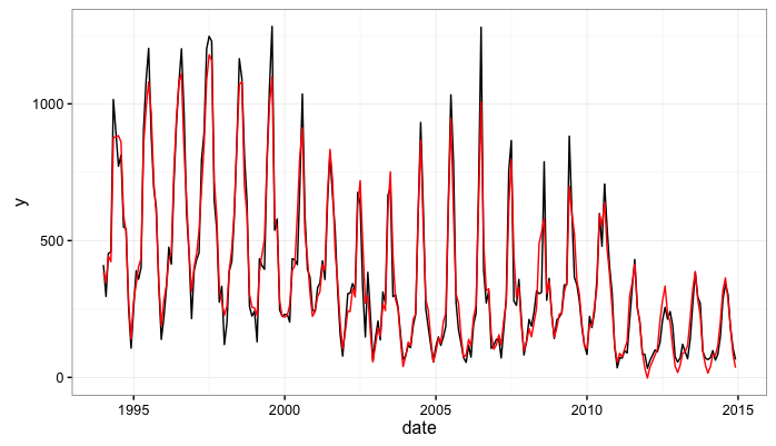
An important thing to note here is that the KFAS package will return both the filtered and smoothed estimates of the state. To get estimates of the seasonal factors which are comparable to seasonal dummy variable regression parameters we extract the smoothed estimates of the state.
Here, we extract the smoothed estimates of the state (the monthly seasonal components) and plot them. In the code below, the object tripsSmooth$alphahat contains the smoothed state estimates:
\[E(Z_{t}\alpha_{t}|y_{1},...,y_{T})\]#---------------------------------------------------------------------------
#plot the seasonal
trips.sea <- as.numeric(tripsSmooth$alphahat[,2])
plot.df <- data.frame(date=dates,seasonal=trips.sea)
#add a reference point to the seasonal data frame
plot.df <- plot.df %>% mutate(month=month(date),july=ifelse(month==7,1,0))
ggplot(plot.df,aes(x=date,y=seasonal)) + geom_line() +
geom_point(aes(color=factor(july))) + scale_color_manual(values=c('red','black'))+
theme_bw() +
theme(legend.position="none")
#----------------------------------------------------------------------------
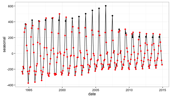
So…first, it’s pretty encouraging that our estimates of the seasonal effect seem to evolve in ways that mirror that our first look at the data. That is, we originally noted that the data seem to exhibit a seasonal peak in July from 1994 to 2010 and also seem to transition to a seasonal peak in August from 2011 - 2014. Our estimate of the seasonal effect obtained from fitting the state-space model also peaks in July in the early parts of the data and moves to a peak in August in the later years of the data.
A Fun Model Comparison Exercise
From the data, we observed (or at least we think we observed) a transition from a July peak to an August peak somewhere around 2010. Another way we could have modeled these data (if, for example we weren’t stoked about the state-space set-up) is with a seasonal dummy variable model and a structural break.
Here, we propose a structural break in 2010 and compare a seasona dummy variable model with a break in 2010 to the state-space model we just fit.
The seasonal dummy variable model with monthly data and a structural break can be formalized as:
\[y_{it} = \alpha + \sum_{i=1}^{11}\gamma_{it}D_{i}Z_{i}\]where $Z_{i}$ is 1 if $t>2010$ and 0 otherwise.
#==========================================================================
#COMPARISON OF THE STATE-SPACE MODEL WITH A DUMMY VARIABLE REGRESSION WITH
# A STRUCTURAL BREAK
#==========================================================================
#get mean absolute error from the KFAS model and compare it to the
# dummy variable model with structural break in 2010.

#the dummy variable model...I know this is clunky but I
# prefer the traditional dummy variable set up.
chow.df <- df.monthly  %>%
            mutate(jan=ifelse(month==1,1,0),
                   feb=ifelse(month==2,1,0),
                   march=ifelse(month==3,1,0),
                   april=ifelse(month==4,1,0),
                   may=ifelse(month==5,1,0),
                   june=ifelse(month==6,1,0),
                   july=ifelse(month==7,1,0),
                   aug=ifelse(month==8,1,0),
                   sept=ifelse(month==9,1,0),
                   oct=ifelse(month==10,1,0),
                   nov=ifelse(month==11,1,0),
                   dec=ifelse(month==12,1,0))

model.pre <- lm(ntrips~feb+march+april+may+june+july+aug+
                  sept+oct+nov+dec+factor(year),data=subset(chow.df,year<=2010))
model.post <- lm(ntrips~feb+march+april+may+june+july+aug+
                   sept+oct+nov+dec+factor(year),data=subset(chow.df,year>2010))

yhat <- rbind(
data.frame(date=chow.df$date[chow.df$year<=2010],
              that=predict(model.pre,newdata=chow.df[chow.df$year<=2010,])),
data.frame(date=chow.df$date[chow.df$year>2010],
           that=predict(model.post,newdata=chow.df[chow.df$year>2010,]))
)

yhat$y <- as.numeric(trips)
yhat$model <- 'Seasonal Dummy'

# the KFAS model
kfas.pred <- data.frame(date=dates,that=fitted(tripsSmooth),y=as.numeric(trips),model='KFAS')

#combine the two
model.comp <- rbind(yhat,kfas.pred)

model.comp$eps <- model.comp$y-model.comp$that

ggplot(model.comp,aes(x=date,y=eps,color=model)) + geom_line() + theme_bw()
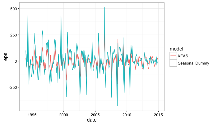
We can compare the mean absolute in-sample prediction error between the two models:
#get mean absolute in-sample prediction error:
tbl_df(model.comp) %>% mutate(abs.error=abs(eps)) %>% group_by(model) %>%
              summarise(mean(abs.error,na.rm=T))

              # A tibble: 2 × 2
           model `mean(abs.error, na.rm = T)`
           <chr>                        <dbl>
1           KFAS                     45.48411
2 Seasonal Dummy                     86.62774