
Average Treatment Effect Examples
Here, I’ve added a bit more substance to an earlier post on quasi-treatement-control methods for social science research. More specifically, I’ve added some content on Propensity Score Matching to the discussion. Enjoy.
Quick procedural note: you can get the data in .csv format via my github repo here.
Introduction
This vignette present a few simple ways to evaluate average treatment effects when some covariates are correlated with both the assignment to treatment and the outcome variable. This is sometimes refered to as sample selection bias or the self selection problem. Let’s consider the example from Matai Cattaneo’s 2010 Journal of Econometrics study of the effect of smoking during pregnancy on babys’ birthweights. The precise empirical problem posed here is that women choose whether or not to smoke, so assignment into treatment and control groups may be non-random. Moreover, the probability of receiving the treatment (smoke v. not smoke) may be correlated with other variables in the model (like age) which are also correlated with the outcome. This is sometimes refered to as a confounding variables problem.
In order to conduct causal inference on the impact of smoking on birthweight we need to estimate the unconditional mean for each group (treatment and control). What we observe is the outcome conditional on receiving the treatment or not. In expirimental studies assignment into treatment-control groups is random and therefore uncorrelated with the outcome. In this case, mean outcomes conditional on the treatment estimate the unconditional mean of interest. In observational studies, if the assignment to treatment-control groups is non-random we need to model this assignment (called the treatment model). If our treatment model is any good than the assignment to treatment conditional on covariates can be considered random and estimates of the unconditional group means can be obtained.
Outline
This workbook illustrates a few approaches for estimating average treatment effects using observational data when self selection into the treatment grouping is a concern:
- The potential outcome mean estimator (POM)
- Comparison of weighted group means using inverse probability weights
- Regression adjustment using propensity scores
Global Options and Data
#load some libraries
library(ggplot2)
library(dplyr)
The data we will use is from from Matai Cattaneo’s 2010 Journal of Econometrics study. These data contain, among other things, measurements on birthweight of 4642 newborn babies, maritial status of the mother, age of the mother, and smoking status (smoked v. did not smoke during pregnancy).
Let’s get a quick look at the data:
df <- tbl_df(read.csv('data/cattaneo2.csv'))
print.data.frame(df[1:5,])
A Motivating Example: Basic Sample Selection Bias Illustration
The estimation of average treatment effects is often complicated by the issue of non-random assignment to treatment and control groups. Here we illustrate this problem using some simulated data on baby’s birthweight and mother’s age and smoker/non-smoker status. In this case, older mothers are more likely to smoke (read: more likely to receive the treatment) but older mothers also tend to give birth to heavier babies.
#generate some data to illustrate the potential observed mean, probability of being a
# smoker increases with age
age=rnorm(100,30,5)
#make the probability that a mother smokes increase with age
psmoke <-  pnorm((age-mean(age))/sd(age))
smoke <- rbinom(100,1,psmoke)
#create a dataframe where birthweight is an increasing function of mother's age and smoking status
z <- data.frame(age=age,smoke=smoke,bw=3000+(5*age)+(25*smoke) + rnorm(100,100,25))
#plot birthweight for smokers and non-smokers
ggplot(z,aes(x=age,y=bw,color=factor(smoke))) + geom_point() + geom_smooth(method='lm') + ylab("birthweight") +
  xlab("mother's age") + scale_color_discrete(name="Smoker") + theme_bw()
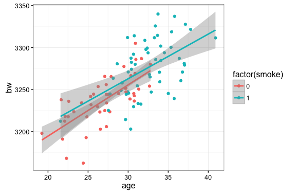
If we are interested in an unbiased estimate of the impact of smoking on birthweight the plot above suggests some issues…namely that we don’t have very many smokers on the low end of the age distribution and, relatedly, we don’t have many non-smokers in the high end of the age distribution.
Potential Outcome Mean (POM) Estimator:
One way researchers have concocted to deal with this phenomenon is to use the Potential Outcome Mean (POM) estimator. This basically amounts to running an OLS regression for each subsample of the data (smokers and non-smokers), using the coefficients of each regression to generate fitted values for the entire data sample, then comparing the means for each set of fitted values. That was convoluted….an example will probably clarify things:
lm.smoker <- lm(bweight~mage,data=df[df$mbsmoke=='smoker',])
pred.smoker <- predict(lm.smoker,newdata=df)
mean(pred.smoker)
[1] 3132.374

lm.ns <- lm(bweight~mage,data=df[df$mbsmoke!='smoker',])
pred.ns <- predict(lm.ns,newdata=df)
mean(pred.ns)
[1] 3409.435

#ATE using the POM approach is just the difference in mean fitted values for smokers and non-smokers
# using the two different regression models
ate <- mean(pred.smoker)-mean(pred.ns)
ate
[1] -275.2519
It’s important to note here that the pattern in the actual data (from Cattaneo 2010) is different from the one we simulated earlier (namely, in the actual data, younger mothers are more likely to smoke).
Propensity Score Corrections
Another popular way of correcting for non-random assignment to treatment/control groups is to use propensity score weighting.
The propensity score is basically the estimated probability that an individual with certain characteristics will receive the treatment. We do this in two parts: first we estimate a model that predicts the probability that each invidual will be included in the treatment group conditional on some covariate values. This is generally called the Treatment Model.
In general, the Treatment Model can be specified many ways. In this application we specify a probit model where the binary outcome, ‘smoker’ is modeled as function of age:
\[P(Y=1|Age) = \Phi(\alpha + \beta age)\]where $\Phi$ is the cumulative density function for the standard normal distribution.
Inverse Probability Weighting Estimating…using the propensity score
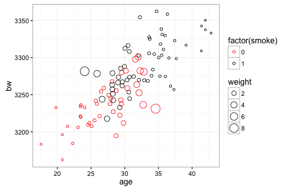
The idea here is pretty simple: we are going to weight observations according to the inverse of thier probability of being included in the sample. Outcomes from smokers will be weighted by $\frac{1}{p_i}$. In the plot below we can see that this will attach a higher weight to outcomes from younger smokers. Conversely, we will weight outcomes from non-smokers by $\frac{1}{1-p_i}$…this attaches a higher weight to older non-smokers. In our simulated data sample is skewed by the fact that older mothers are more likely to smoke and more likey to have heavier babies. The inverse probability weight correction deals with this by attaching higher weights to observations that are underrepresented in the sample (non-smoking older mothers and smoking younger mothers).
#start with the same fake data we used to illustrate the POM estimator
age=rnorm(100,30,5)
psmoke <-  pnorm((age-mean(age))/sd(age))
smoke <- rbinom(100,1,psmoke)
z <- data.frame(age=age,smoke=smoke,bw=3000+(5*age)+(25*smoke) + rnorm(100,100,25))

#calculate probability weights: fit a logit model and probit then use the fitted values as
# probabilities
logit.bw <- glm(smoke~age,data=z,family='binomial')
probit.bw <- glm(smoke~age,data=z,family=binomial(link='probit'))
pi <- predict(probit.bw,newdata=z,type="response")

#weight smokers by 1/p(i) so that weight is large when probability of being a smoker is
# small.  Weight observations on non-smokers by 1/(1-p(i)) so weights are large when
# probability is small
z <- tbl_df(z) %>% mutate(w=pi) %>%
    mutate(weight=ifelse(smoke==1,1/w,1/(1-w)))

ggplot(z,aes(x=age,y=bw,color=factor(smoke),size=weight)) + geom_point(shape=1) +
  scale_color_manual(values=c("red","black"))
In the following chunk we estimate the Average Treatment Effect with our Cattaneo (2010) data using the inverse probability weights to adjust the means:
#Treatment Model
#use the probit link for probability weights like they do in the STATA blog
probit.bw <- glm(mbsmoke~mage,data=df,family='binomial'(link='probit'))
pi <- predict(probit.bw,newdata=df,type="response")

#add inverse probability weights to the data frame
df <- tbl_df(df) %>% mutate(w=pi) %>% mutate(weight=ifelse(mbsmoke=='smoker',1/w,1/(1-w)),
                                             z=ifelse(mbsmoke=='smoker',1,0))

#Average Treatment Effect based on weighted average of groups:
#Reference: http://onlinelibrary.wiley.com/doi/10.1002/sim.6607/epdf
weighted.mean.smoker <- (1/(sum(df$z/df$w)))*sum(df$z*df$bweight/df$w)
weighted.mean.ns <- (1/sum(((1-df$z)/(1-df$w))))*(sum(((1-df$z)*df$bweight)/(1-df$w)))

#ATE
weighted.mean.smoker - weighted.mean.ns
[1] -275.5007
Propensity Score Regression Adjustment
We can also use the propensity score as a regression adjustment. A good reference for this estimator is this post on Andrew Gelman’s Blog.
Using the propensity score as a regression adjustment simply amounts to including the propensity score ($p_i$) in a regression of birthweight on mother’s age.
In the chunk below the treatment model is specified as a probit model where the [0,1] outcome smoker v. non-smoker is modeled as a function of age, age squared, marital status, education level, and an indicator for whether the mother has had a baby before. Parameter estimates from this model are used to generate a predicted probability of smoking for each individual in the sample. This predicted probability is the propensity score.
#the treatment model
pscore.df <- df %>% mutate(mage2=mage*mage) %>%
        mutate(marriedYN=ifelse(mmarried=='married',1,0),
               prenatal1YN=ifelse(prenatal1=='Yes',1,0))

ipwra.treat <- glm(factor(mbsmoke)~mage+marriedYN+fbaby+mage2+medu,data=pscore.df,family='binomial'(link='probit'))
pi <- predict(ipwra.treat,newdata=pscore.df,type="response")
df$ipwra.p <- pi
pscore.df <- df %>% mutate(ipwra.w=ifelse(mbsmoke=='smoker',1/ipwra.p,1/(1-ipwra.p)))

#Birthweight regression adjusted using the propensity score
summary(lm(bweight~factor(mbsmoke)+ipwra.p,data=pscore.df))

Call:
lm(formula = bweight ~ factor(mbsmoke) + ipwra.p, data = df)

Residuals:
     Min       1Q   Median       3Q      Max
-3099.51  -313.05    23.66   352.16  2023.94

Coefficients:
                      Estimate Std. Error t value Pr(>|t|)
(Intercept)            3510.18      15.75 222.852  < 2e-16 ***
factor(mbsmoke)smoker  -226.88      22.25 -10.197  < 2e-16 ***
ipwra.p                -572.52      75.26  -7.607 3.36e-14 ***
---
Signif. codes:  0 ‘***’ 0.001 ‘**’ 0.01 ‘*’ 0.05 ‘.’ 0.1 ‘ ’ 1

Residual standard error: 565.4 on 4639 degrees of freedom
Multiple R-squared:  0.04616,	Adjusted R-squared:  0.04575
F-statistic: 112.3 on 2 and 4639 DF,  p-value: < 2.2e-16
Propensity Score Matching
The intuition and mechanics of Propensity Score Matching are pretty simply to understand. The statistical foundations (i.e. how to do PSM right) are pretty complex. My understanding of causal inference doesn’t come close to a Paul Rosenbaum, Don Rubin, Andrew Gelman, or Judea Pearl…so I’m not going to preface this discussion of PSM with a lot of cautionary tales. I’m not going to run through a big list of ‘potential pitfalls’ or common violations of the ignorability condition. I’m just going to walk through the nuts-and-bolts of how to take our birthweight data and estimate an average treatment effect using PSM.
But since I’m not providing a bigger discussion of technical minutia let me offer this advice: if any of you are considering using Propensity Score Matching Models in any serious application you should first:
- Read Rosenbaum and Rubin 1983
- Read Judea Pearl’s Causality…yes, the whole thing…but if not the cover-to-cover than at least Chapter 11 where Propensity Score Matching is specifically addressed.
- Read Andrew Gelman’s thoughts on causality and PSM…this is a good place to start
A typical propensity score matching application goes something this:
- run a probit or a logit regression modeling the assignment to treatment $z /in (0,1)$ as a function of covariates $x$.
- using the regression in 1, generate a predicted probability of receiving the treatment for each observation in the sample.
- match treated units to untreated units using the propensity score. NOTE: there are a number of options for carrying out this matching (many-to-one match, one-to-many match, one-to-one match, nearest neighbor match, Mahalanobis distance, etc.)
- examine the covariate balance in the matched data…interestingly, there seem to be a rash of PSM applications that don’t offer much advice in way of what to do if your model doesn’t provide good covariate balance.
- compare group means in the matched data.
Step 0: read in the data…I know this is a little repetitive…I should probably clean this up but for now just live with it please.
library(MatchIt)
#read the Cattaneo2.dta data set in
df <- tbl_df(read.csv("data/cattaneo2.csv")) %>%
      mutate(smoker=ifelse(mbsmoke=='smoker',1,0))
Steps 1 and 2: run the logit model and get the predicted probability of receiving the treatment (propensity score).
#use mother's age, marital status, and education level to predict smoke/non-smoke
smoke.model <- glm(smoker~mage+medu+mmarried,family=binomial, data=df)

pr.df <- data.frame( pr_score = predict(smoke.model, type = "response"),
                      smoke = df$smoker )
Step 3: use the ‘MatchIt’ package to match treated units to similar non-treated units
#The 'MatchIt' package will perform the actual propensity score matching for us:
m.out <- matchit(smoker ~ mage + medu + mmarried,
                 method = "nearest", data = df)

#match.data creates a dataframe with only the matched obs
matched <- match.data(m.out)
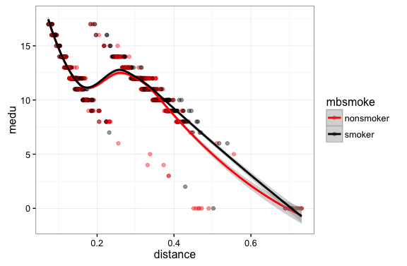
Step 4: examine the covariate balance. In a good PSM study the covariate distributions conditional on propensity score should be similar across groups.
#inspect the covariate balance
ggplot(matched,aes(x=distance,y=mage,color=mbsmoke)) + geom_point(alpha=0.4,size=1.5) + geom_smooth() +
  theme_bw() + scale_color_manual(values=c('red','black'))

ggplot(matched,aes(x=distance,y=medu,color=mbsmoke)) + geom_point(alpha=0.4,size=1.5) + geom_smooth() +
  theme_bw() + scale_color_manual(values=c('red','black'))
Step 4A: inspect covariate balance using a t-test of means
#t-test of means
t.test(matched$mage[matched$mbsmoke=="smoker"],matched$mage[matched$mbsmoke!="smoker"])

	Welch Two Sample t-test

data:  matched$mage[matched$mbsmoke == "smoker"] and matched$mage[matched$mbsmoke != "smoker"]
t = 0.23643, df = 1708, p-value = 0.8131
alternative hypothesis: true difference in means is not equal to 0
95 percent confidence interval:
 -0.4644314  0.5917462
sample estimates:
mean of x mean of y
 25.16667  25.10301


t.test(matched$medu[matched$mbsmoke=="smoker"],matched$medu[matched$mbsmoke!="smoker"])

	Welch Two Sample t-test

data:  matched$medu[matched$mbsmoke == "smoker"] and matched$medu[matched$mbsmoke != "smoker"]
t = 0.96778, df = 1708.4, p-value = 0.3333
alternative hypothesis: true difference in means is not equal to 0
95 percent confidence interval:
 -0.1093186  0.3222815
sample estimates:
mean of x mean of y
 11.63889  11.53241
Step 4C: inspect the covariate balance using average absolute standardized difference….I plan to add this a little later….for now have a look at Simon Ejdemyr’s PSM tutorial.
Step 5: Finally, to get the average treatment effect from our PSM set-up, we compare the grouped means in the matched sample:
with(matched, t.test(bweight ~ mbsmoke))

	Welch Two Sample t-test

data:  bweight by mbsmoke
t = 6.9866, df = 1704.9, p-value = 4.023e-12
alternative hypothesis: true difference in means is not equal to 0
95 percent confidence interval:
 143.8564 256.1505
sample estimates:
mean in group nonsmoker    mean in group smoker
               3337.663                3137.660