This is a little bit of rehash of an earlier post on President Cheeto Jesus’ economic agenda. The core message is basically the same, but the supporting evidence has been vastly simplified.

Research Question:

Followers of the Angry Tangerine seem to believe that cutting the corporate tax rate will lead to rainbow stew and blow jobs all around for Blue Collar America. Is there any sensible basis for this expectation?

Methods

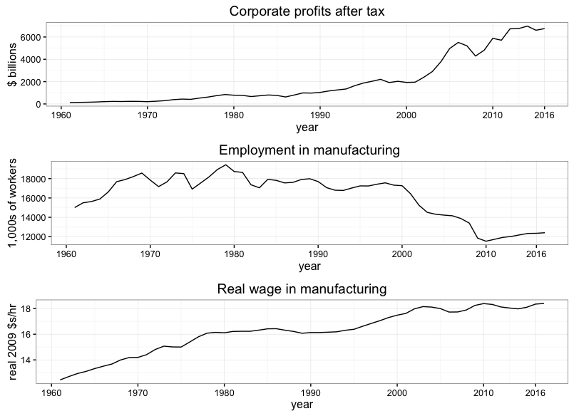
Plot corporate profits, manufacturing employment, and wages in manufacturing together and look at them. If we lower the corporate tax rate we expect corporate profits after tax to rise. By plotting corporate profits after tax over time along with manufacturing employment and earnings we can visualize whether historical increases in corporate profits were positively correlated with increases in either manufacturing employment or earnings.

Basically, we’re asking, when corporations make more money do they hire more blue collar workers or do they pay existing workers more?

Innovation over my previous post

Rather than monkey around with downloading data from the Federal Reserve Bank of Saint Louis’s FRED database to a bunch of .csv files and loading those into R, I’m going to use the Quantmod package in R to pull data series directly from FRED.

Results

library(quantmod)
library(dplyr)
library(lubridate)


#nominal hourly earnings in manufacturing (monthly)
getSymbols("CES3000000008",src='FRED')

#GDP deflator
getSymbols("GDPDEF",src='FRED')

#----------------------------------------------------
#real hourly earnings in manufacturing

man.wage <- tbl_df(data.frame(date = index(CES3000000008), 
           nom.wage=CES3000000008, row.names=NULL)) %>%
            mutate(w.man=CES3000000008,year=year(date),month=month(date)) %>%
            group_by(year) %>% 
            summarise(w.man=mean(w.man)) 

deflator <- tbl_df(data.frame(date=index(GDPDEF),def=GDPDEF)) %>%
             mutate(year=year(date),month=month(date)) %>%
             group_by(year) %>% 
             summarise(def=mean(GDPDEF)) %>%
             inner_join(man.wage,by=c('year'))
  
base <- deflator$def[which(deflator$year == 2009)]

deflator <- deflator %>% mutate(real.wage=w.man/(def/base))
(log(deflator$real.wage[deflator$year==2016])-log(deflator$real.wage[deflator$year==2000]))/16

manwage.plot <- ggplot(subset(deflator,year>1960),aes(x=year,y=real.wage)) + geom_line() +
  theme_bw() + ylab("real 2009 $s/hr") + ggtitle("Real wage in manufacturing") + 
  scale_x_continuous(breaks=c(1960,1970,1980,1990,2000,2010,2016))


#----------------------------------------------------


#-----------------------------------------------------
getSymbols("MANEMP",src='FRED')

manemp <- tbl_df(data.frame(date=index(MANEMP),manemp=MANEMP)) %>% 
           mutate(year=year(date),month=month(date)) %>%
           group_by(year) %>% summarise(manemp=mean(MANEMP))

manemp.plot <- ggplot(subset(manemp,year>1960),aes(x=year,y=manemp)) + geom_line() + 
  theme_bw() + ylab('1,000s of workers') + ggtitle('Employment in manufacturing') +
  scale_x_continuous(breaks=c(1960,1970,1980,1990,2000,2010,2016))


#-------------------------------------------------------


#-------------------------------------------------------
#corporate profits after tax

getSymbols("CP",src='FRED')
cp <- tbl_df(data.frame(date=index(CP),cp=CP)) %>%
      mutate(year=year(date),month=month(date)) %>%
      filter(year < 2017) %>%
      group_by(year) %>% summarise(cp=sum(CP))

cp.plot <- ggplot(subset(cp,year>1960),aes(x=year,y=cp)) + geom_line() + 
  theme_bw() + ylab('$ billions') + ggtitle('Corporate profits after tax') + 
  scale_x_continuous(breaks=c(1960,1970,1980,1990,2000,2010,2016))
(log(cp$cp[cp$year==2016])-log(cp$cp[cp$year==2000]))/16
#-------------------------------------------------------


#------------------------------------------------------
require(gridExtra)

grid.arrange(cp.plot, manemp.plot, manwage.plot, ncol=1)

Discussion

If you’re sitting there thinking, this seems like a complicated issue, there’s probably more to the relationship between corporate taxation and employment and wages then can be exhaustively examined in a few plots showing correlations over time, I don’t blame you. And you’re probably right. This probably is a complex issue. It probably does warrant a deeper dive than just appropriating some plots from the St. Louis Fed’s macroeconomic database.

But if you were inclined to think,

Yeah man, cut corporate taxes, give them more money and they’ll hire more people. Easy peesy lemon squeezy

then you probably need to have a come-to-Jesus with some basic facts about our economy:

Between 2000 and 2016,

• Corporate profits grew at an average rate of 7.8% per year
• Real wages in manufacturing grew at an average rate of less than 1% per year
• Employment in manufacturing declined at an average rate of 2% per year

Final Words

This is not meant to be the end of this discussion. These are just plots that are pretty easy to make, pretty easy to digest and pretty clearly demonstrate the need for some skepticizm regarding the benefit to ‘working class Americans’ of cutting the corporate tax rate.

If you think I’m wrong and you’re still convinced that cutting the corporate tax rate will be amazing for working class Americans just give me a convincing answer to the following question:

If you’re so sure that corporations are going to respond to a tax cut by hiring more workers and pay everybody like it’s Christmas then why didn’t they do that with any of thier windfall profits over the last 16 years?