Sqlite and rsqlite
I had occassion to setup an SQLite database the other day. I found it be a most enjoyable experience so I thought I’d share. In this short post I’ll:
- use the Mac Terminal and sqlite shell to set up a local embedded database
- use the RSQLite package to access database tables from R.
Background
I joined Kaggle’s Data Science for Good: Donors Choose challenge. The purpose of the challenge is to develop a data analytics methodology to help the education non-profit site Donors Choose increase contributions to public school classrooms.
Problem Statement
This first pinch-point I encountered with this challenge was that the data were made available as as series of very large .csv files. This was making even the elementary task of running summary stats and just ‘getting a feel’ for the data cumbersome and time consuming. For instance:
- one of the data files that contained info on donations (Donations.csv) to past project was about 500 MB and took about 4 minutes just to load into an R workspace using the read.csv() method.
- the data file with information about individual projects (Projects.csv) was 2.2 GB and took almost 10 minutes to bring into R using the read.csv() method.
Note: the data files are available for download here
Solution
Since I don’t really need all 4 million observations in the Donations.csv data or all 2 million observations in the Projects.csv file in order to ‘get a feel’ for the data, I shoved the data files into a relational database that I could query for smaller chunks of data.
Execution
Step 1: create a database
I did this using the sqlite shell and I established the database in the directory that was previously set up for this R Studio Project:
cd Users/aaronmamula/Documents/R projects/kaggle/donors-choose/data
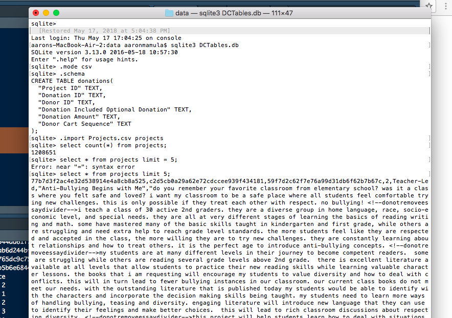
aarons-MacBook-Air-2:data aaronmamula$ sqlite3 DCTables.db
SQLite version 3.13.0 2016-05-18 10:57:30
Enter ".help" for usage hints.
Step 2: load .csv files into database as DB tables
sqlite> .mode csv
sqlite> .import Projects.csv projects
sqlite> select count(*) from projects;
1208651
Step 3: Pull data from the DCTables database into R
If DBI and RSQLite are not yet installed on your R instance then install them.
library(DBI)
library(RSQLite)

con = dbConnect(SQLite(), dbname="data/DCTables.db")
dbGetQuery(con, 'SELECT * FROM donations LIMIT 5')
                        Project ID                      Donation ID                         Donor ID
1 000009891526c0ade7180f8423792063 5a032791e31167a70206bfb86fb60035 6d5b22d39e68c656071a842732c63a0c
2 000009891526c0ade7180f8423792063 38d2744bf9138b0b57ed581c76c0e2da 377944ad61f72d800b25ec1862aec363
3 000009891526c0ade7180f8423792063 dcf1071da3aa3561f91ac689d1f73dee 4aaab6d244bf3599682239ed5591af8a
4 000009891526c0ade7180f8423792063 18a234b9d1e538c431761d521ea7799d 0b0765dc9c759adc48a07688ba25e94e
5 000009891526c0ade7180f8423792063 688729120858666221208529ee3fc18e 1f4b5b6e68445c6c4a0509b3aca93f38
  Donation Included Optional Donation Donation Amount Donor Cart Sequence
1                                 Yes              25                   2
2                                 Yes              25                   1
3                                 Yes              25                   2
4                                 Yes              20                   3
5                                  No          178.37                  11
In addition to efficiencies related to the ability to bring only certain parts of a data table into R, using the RSQLite package I can also load an entire table in a fraction of the time it takes to load the same table from a .csv file.
t <- Sys.time()
donations <- read.csv('data/Donations.csv')
Sys.time() - t
Time difference of 3.542474 mins

t <- Sys.time()
test <- dbGetQuery(con,'SELECT * FROM donations')
Sys.time() - t
Time difference of 30.18701 secs
Also, R doesn’t really mind long-narrow data (millions of rows of one or two variable) but gets pretty finicky about wide data (lots of columns). Bring data in from a database provides a nice way to do elementary summary stats if you have just a few variable of interest because you can pull out just a column or two:
amts <- dbGetQuery(con,'SELECT "Donation Amount" FROM donations')
nrow(amts)
[1] 4855240
summary(as.numeric(amt$donation_amount))
    Min.  1st Qu.   Median     Mean  3rd Qu.     Max.     NA's
    0.00    14.85    25.00    60.66    50.00 60000.00   184860
Bonus Ball
Since I’ve got these data into a workspace now, let’s join the donations data and projects data and do a couple first pass data summary tasks:
#-----------------------------------------------------------------------
#summarise project donations and merge with projects data to see
# how many projects got close to their goal

donations <- dbGetQuery(con,'SELECT * FROM donations')
names(donations) <- c('project_id','donation_id','donor_id','donation_included_optional_donation',
                 'donation_amount','donor_cart_sequence')

proj.donations <- test %>% group_by(project_id) %>%
                      summarise(ndonations=n_distinct(donation_id),
                                ndonors=n_distinct(donor_id),
                                total_donations=sum(as.numeric(donation_amount),na.rm=T),
                                average_donation=mean(as.numeric(donation_amount),na.rm=T))

project <- dbGetQuery(con,'SELECT "Project ID", "School ID", "Teacher ID",
                      "Teacher Project Posted Sequence", "Project Type", "Project Title",
                      "Project Grade Level Category", "Project Resource Category",
                      "Project Cost", "Project Posted Date", "Project Current Status",
                      "Project Fully Funded Date" FROM projects')

names(project) <- c('project_id','school_id','teacher_id','teacher_project_posted_sequence',
                    'project_type','project_title','project_grade_level_category',
                    'project_resource_category','project_cost','project_posted_date',
                    'project_current_status','project_fully_funded_date')

project <- project %>% left_join(proj.donations,by=c('project_id'))
#-------------------------------------------------------------------------
How many projects in our data got no contributions?
> nrow(project)
[1] 1208651
> nrow(project[is.na(project$ndonations),])
[1] 309632
So about 300,000 projects in the database did not get any contributions
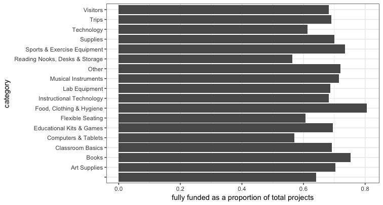
What is the distribution of project types for fully funded projects
cat <- project %>%
          mutate(fully_funded=ifelse(project_current_status=='Fully Funded',1,0)) %>%
           group_by(project_resource_category) %>% mutate(total_count=n()) %>%
          group_by(project_resource_category,fully_funded)  %>%
           summarise(count=n(),total=max(total_count)) %>%
          mutate(funded.pct = count/total) %>%
          filter(fully_funded==1)

ggplot(cat,aes(x=project_resource_category,y=funded.pct)) + geom_bar(stat='identity') +
  coord_flip() + theme_bw() + xlab('category') +
  ylab('fully funded as a proportion of total projects')