I built my first R Shiny app. It’s laughably simple but, in this case, I think the simplicity will make for a good first blog post on R Shiny.

The Shiny package for R provides a really easy and cool way to make interactive apps. I’ve seen a lot of really cool sophisticated data analytics apps built with Shiny. There are a lot of cool examples that you can check out in the app gallery here. Another set of Shiny apps I recommend checking out are bundled in a project called the Fisheries Economics Explorer.

Pre-reqs

1. get data file called gf_monthly.RDA from my github repository
2. make sure you have the ‘shiny’ package installed and loaded in R

Game plan

My overarching goal for this simple proof-of-concept app is to have a process that:

1. allows a user to select from different models, model classes, or modeling assumptions available for analysis of a time-series
2. apply the users’ selections to the time-series and output a visual display of the analysis
3. allow the output to be reactive in the sense of allowing the users to update in real time any of the chosen inputs and have the output update accordingly.

What I have accomplished so far is just a very simple starting point. The current app does the following:

1. loads a data set of commercial fishing trips taken by month off the U.S. West Coast from Jan-1994 to Aug-2016

2. allows the user to choose either a Kalman Filter-based state space model or a simple linear regression with annual and seasonal (monthly) fixed effects

3. outputs a plot of the original data and the in sample predictions of the chosen model. For the Kalman Filter the in-sample predictions are based on the smoothed state estimates. For the linear model the in-sample predictions are just the fitted values given by the linear predictor:

What I would like to add to this starter app is:

1. Add more models to choose from

2. Add more output options….basically more diagnotics (error checking) and final outputs (out-of-sample forecasts)

Here’s my app:

df.monthly <- readRDS("gf_monthly.RDA")
df.monthly <- tbl_df(df.monthly) %>% filter(year<2016) %>%
               mutate(date=as.Date(paste(df.monthly$year,"-",df.monthly$month,"-","01",sep=""),
                                   format="%Y-%m-%d"))
library(KFAS)
library(xts)
library(mgcv)

ui <- fluidPage(
  headerPanel('Fishing Trips'),
  sidebarPanel(
    selectInput('model', 'Model', c('State Space Model','Linear Model')),
    numericInput('startyr', 'Start Year', 1996,
                 min = 1994, max = 1998)
  ),
  mainPanel(
    plotOutput('plot1')
  )
)

server <- function(input, output) {
 
  trips <- reactive({
    df.monthly %>% filter(year >= input$startyr) %>% select(date,ntrips,month,year)
  })
     

  pred <- reactive({
    fitted(KFS(fitSSM(SSModel(xts(trips()$ntrips,order.by=trips()$date) ~ 
              SSMtrend(degree = 1, Q=list(matrix(NA))) + 
              SSMseasonal(period=12, sea.type="dummy", Q = NA), H = NA),
            inits=c(0.1,0.05, 0.001),method='BFGS')$model,
                    smooth= c('state', 'mean','disturbance')))
            
  })                                       
  
  results <- reactive({ 
    r <- data.frame(y=trips()$ntrips,x1=trips()$month,x2=trips()$year)
  })
  
  lmod <- reactive ({ 
    mod1 <- predict.lm(lm(y~factor(x1)+factor(x2), data = results() ) )
  })
  
  plotdf <- reactive({
    if(input$model=='State Space Model'){
      data.frame(
        rbind(
          data.frame(date=trips()$date,ntrips=trips()$ntrips,model='observed'),
          data.frame(date=trips()$date,ntrips=pred(),model='Seasonal SSM')
        )
      )
      }else{
       data.frame(
         rbind(
           data.frame(date=trips()$date,ntrips=trips()$ntrips,model='observed'),
           data.frame(date=trips()$date,ntrips=lmod(),model='Seasonal OLS')
         )
       )
      }
    
    
    })
  
    output$plot1 <- renderPlot({
      ggplot(plotdf(),aes(x=date,y=ntrips,color=model)) + geom_line() + 
                   theme_bw() + scale_color_manual(values=c('blue','black'))
  })
    

}

shinyApp(ui = ui, server = server)

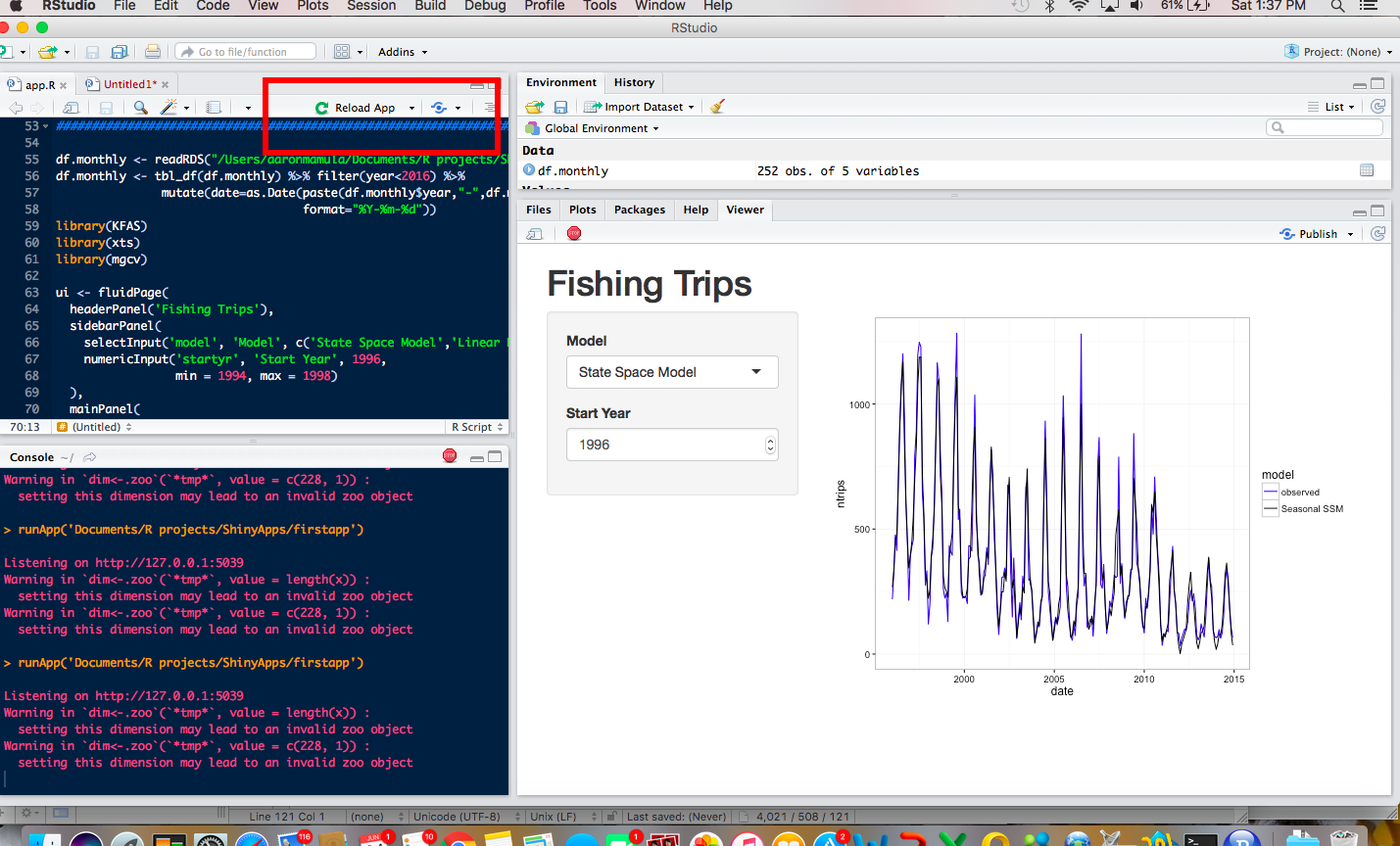
Here’s a static image of what it looks like when I run it in an R Studio Viewer Pane:

Try it out

You can mess around with my app on the web here. In addition to web interaction, you can run my code (provided you have the ‘Shiny’ library installed and you get the gf_monthly.RDA file off of my github repo) in R Studio and the app will pop up in either a local browser tab or inside R Studio (depending on how you configure things).

You can toggle between model types (currently your only options are ‘State Space Model’ and ‘Linear Model’) and set a few different starting years that can define the range of the data you want to display.

I really like the option to run the app in an interactive viewer pane inside R Studio so I’ll take a quick second and show you how to do that:

1. make sure the file containing your shiny code is saved in a file called “app.R”. As long as the file has that exact name, R Studio will recognize it as a Shiny app and will give you options for how to display it.

2. in the image below notice that R Studio has recognized the code as a Shiny app and provided an options bar at the top right portion of the scripting window. That options bar will allow to chose whether to run the app in an R Studio viewer pane, publish it to an R Shiny Server, or run it in a local browser window.

Motivation

I really like the idea of using interactive apps to help communicate uncertainty. An important function of my job is providing science advice to policy and decision makers (what I loosely call ‘decision support’). Whether its scientists providing analysis to help legislators make informed choices about public policy options or data scientists providing analysis to upper level managers in support of some business question, we all face a fundamental tension between providing useable advice and being honest and transparent about the limitations of our analysis.

In oversimplified terms this tension arises because decision makers (politicians, policy makers, business managers, executive) want clear guidance on how to proceed on important issues. Analysts want to provide clear guidance but also want high level decision makers to understand the pros and cons of the options available to them and take some ownership over the ultimate decision.

I don’t want to get into a whole thing about uncertainty. It’s a super interesting topic but also very complex topic. I do want to mention that any empirical analysis generally has to include a coherant strategy for dealing with uncertainty. In statistical analysis uncertainty can arise in the following forms:

• we have errors that can arise because our inability to precisely and accurately measure things
• we have errors that can arise because statistical randomness makes it difficult/impossible to know how well a sample of data represents a bigger population
• we can have errors in parameter estimation that can arise because of the stochastic nature of the data.

In addition to these types of scientific uncertainty, analysts face another type of uncertainty associated with our inability to observe the decision makers’ preferences.

Example 1 Public policy options often have distributional consequences. If we think about a really simple way to break down a proposed increase in the minimum wage, we might assume that:

• people who hire minimum wage works will be incentivized to substitute capital for labor (hire more computers and fewer workers)
• minimum wage workers will decrease in number but each worker will take home more money
• consumers may higher prices for some things.

In this case the overall impact of the policy will be moved by the magnitudes of these three effects. Even if the magnitudes are such that the overall project produces substantial total benefits (when evaluated across all impacted parties), policies makers might have different preference and risk tolerances for impacts to specific groups. In this case, it will be important to characterize (possibly under a few scenarios) who wins, who loses, how much the winners win, how much the losers lose. This is exactly the type of thing that I think R Shiny interactive applications could be really good for….instead of giving the decision maker a 100 page report detailing the model, assumptions, estimation strategy, total estimated benefits, and expected distributions of benefits and costs across different parties, we could give them a web application that allows them to interact with the key features of the analysis and visualize how these feature change whatever outputs the decision makers care most about.

Example 2 Financial analysis generally involves matching expected outcomes with the risk tolerance of the decision maker. It’s pretty easy to imagine 3 portfolio options that have: 1. high risk with potential for high return, 2. medium risk with mid-level return, and 3. low risk with consistent but modest return.

From what I’ve seen of R Shiny so far, I think it could be a really useful tool for helping analysts convey the range of options and possible consequences of each option to decision makers. In my experience, decision makers don’t really want to see hundreds of pages of sensativity analysis and scenario analysis. They want analysis that can be distilled down to something digestable. In contrast, analyst who have undertaken a careful analysis that is influenced by different types of uncertainty and affected by modeling assumptions, want people to understand the nuance of their analysis before running off to apply it. I think the interactive nature of R Shiny apps could really help establish the middle ground between these two end.