Model-free quantification of time-series predictability

I read an interesting paper recently. I wrote a half-ass review of it here. Below I provide some notes and interesting nuggets I took from my reading of “Model-free quantification of time-series predictability” by Garland, Jame, and Bradley, published in Physical Review v. 90:

Executive Summary

Here are the main points and maybe a few things to think about as you read on:

Permutation Entropy is pretty cool. Basically, ‘complexity’ of a time-series can be evaluated in terms of repetition. That is by asking, how often do patterns of particular lengths repeat in the time-series? Permutation entropy is a measure of repetition. It provides a way of simplifying a time-series by using symbolic dynamics and looking for patterns in the simplied series.
A lot of the stuff in the paper was pretty new to me. My experience with Quantitative Ecology and Mathematical Biology is that sometimes things sound new and exciting to me because they use different words for things that I actually find old and boring…and sometimes things sound new and exciting because Ecologists and Biologists are grappling with problems that have differnt features, constraints, or dimensions than problems typically considered in the Social Sciences…I probably need to read a few more papers in the ‘Complexity Theory’ strand of literature to know where this stuff falls.
I still have yet to play around with the different tuning parameters used in complexity metrics like Permutation Entropy. I’m hoping to do some of this soon, but at the moment I’m still a bit hazy on the role of ‘word length’ or the maximum permuntation length.

Some paper specific issues that might be interesting to others:

A much more experienced time-series analyst in the reading group pointed out that for a handful of time-series that we generated in our group meeting, the Weighted Permutation Entropy had no notable relationship to the maximum Lyapanov Exponent….I don’t spend a lot of time with chaotic dynamics so I’m not all that confident in my understanding of Lyapanov Exponents but this divergence was generally viewed as unsettling.
The abstract of the paper in question hinted that one implication of this line of inquiry (‘model-free quantification of predictability’) was that one could make some inferences about what class of time-series model was likely to yeild the best predictions for time-series exhibiting different “complexities.” If the authors did indeed make some commentary on this subject, they managed to hide it quite well. I read the paper 3 times and didn’t pick up much in the way of evaluating potential for different time-series models to perform in different “complexity” paradigms.

Background

My lab has a small ‘quantitative methods’ reading group that meets every Thursday (I’m somewhat ashamed to admit that we, rather arrogantly, call ourselves ‘math club’). The idea is to focus on emerging topics in math/statistics/estimation/modeling/etc that might be applicable across disciplines. Since I work primarily with physical and biological scientists, the papers we read tend to have an ecological bent (Journal of Statistical Physics, Applied Ecology, and Ecology Letters tend to be rich sources for this reading group). Because of this bent, and the fact that I’m around Ecologists/Biologist/Hydrologists/Geneticists all day (and seldom around Economists), I usually use my blogging time for more pure ‘Econ’ related pursuits.

However, yesterday’s paper kind of hit on the time-series theme that I’ve been blogging about lately so I thought it might be worth reviewing.

The paper:

Model-free quantification of time-series predictability

A supporting reference:

Practical consideration of permutation entropy: A tutorial review

The General Idea

This paper focuses on the relationship between complexity of a time-series and predictability. My interpretation of what the authors are focusing on is the following: can we measure how much structure exists in a particular time-series that may be exploited in order to make good prediction (if we had the correct model)?

An aside: I found the paper philosophically interesting because it was really trying to operate in the ‘model free’ environment. That is, I read a lot of papers that explore strengths and weakness of different models leveraged for different purposes. This paper was less interested in identifying the ‘right’ model and more interested in the question of, “can even the best model accurately predict values in a time-series?” This appears to be a more active area of research than I realized. I thought this question was quite novel, turns out it’s been under investigation for some time.

The Set Up

The paper proceeded according to the following basic breakdown:

generate several different time-series with different complexity properties - some with simple periodic dynamics, some with highly non-linear and chaotic dynamics.
Use 4 broad classes of models to try and predict out-of-sample observations of each series.
Calculate the Mean Absolute Scaled Prediction Error for each model applied to each time-series. MASE is defined as:

\[MASE=\sum_{j=n+1}^{k+n+1}\frac{|p_{j}-c_{j}|}{\frac{k}{n-1}\sum_{i=2}^{n}|x_{i}-x{i-1}|}\]

Quantify the ‘complexity’ of each time-series. Philosophically, the authors describe complexity as a function of redundancy… practically, the authors argue that weighted permutation entropy is an effective way to measure redundancy.
Evaluate the relationship between prediction error and ‘complexity’ for each model and each time-series.

The four broad classes of model that were used from Step 2 above were:

naive: the naive model basically says the best predictor of $x_{t}$ given $x_{1},…x_{t-1}$ is the average
random walk: a model that says the best prediction of $x_{t}$ is $x_{t-1}$
ARIMA: the auto.arima procedure in R was used to determine the best ARIMA order to predict each time-series
The Lorenz method of analogues….I won’t pretend I know what this is. I don’t.

The Metrics

One of the big things I got out of this paper was the metric of Permutation Entropy for measuring the ‘complexity’ of a time-series. Permutation Entropy is not a new concept/measurement but it was new to me..although saying I was unfamiliar with an arbitrary entropy measure isn’t saying much of an consequence. For whatever reason, I don’t use entropy measures very often in my work.

The overriding idea in this paper is that redundancy in a time-series means that the time-series has some repeating patterns and some structure that - provided one has the right model to capture the underlying dynamics - can be exploited in order to make good predictions about unobserved values in the series. Time-series with little redundancy are ‘complex’ as they have very little structure that can be leveraged. Permutation entropy, or more precisely, weighted permutation entropy is a proxy for redundancy…and therefore a measure of how much structure exists in a time-series and can be exploited in order to forecast.

A Quick Expiriment

I’v only spent a little time trying to ‘roll my own’ permutation entropy code so this is probably really clunky…but, as luck would have it, an R package to do it already exists…it’s called statcomp. I base my R code on the following definition and pseudo-code provided in Practical consideration of permutation entropy: A tutorial review…although I note that I’m pretty sure there are a few errors in the paper.

Basic steps for calculating permutation entropy:

Define the order of permutation n. That leads to the possible permutation patterns $\pi_{j} (j = 1, .., n!)$ which are built from the numbers 1, …, n.
Initialize i = 1 as the index of the considered time series $x_{i}=1,…,N$ and the counter $z_{j} = 0$ for each $\pi_{j}$.
Calculate the ranks of the values in the sequence $x_{i}, …, x_{i+n−1}$ which leads to the rank sequence $r_{i}, …, r_{i+n−1}$. The ranks are the indices of the values in ascending sorted order.
Compare the rank sequence of step 3 with all permutations pattern and increase the counter of the equal pattern $\pi_{k} = r_{i}, …, r_{i+n−1}$ by one $(z_{k} = z_{k} + 1).$
If $i ≤ N − n$ then increase i by one (i = i + 1) and start from step 3 again. If $i>N − n$ go to the next step.
Calculate the relative frequency of all permutations $/pi_{j}$ by means of $p_{j} = \frac{z_{j}}{z_{k}}$ as an estimation of their probability $p_{j}$ .
Select all values of $p_{j}$ greater than 0 (since empty symbol classes $0 log(0) = 0$) and calculate the permutation entropy.

Pseudo Code for calculating permutation entropy:

This pertains to a specialized case. For the generalized process please refer to the paper.

Consider the time-series x=[6,9,11,12,8,13,5] which has N=7.

Step 1: The permutation order is set to n=3 and so n! is 6. The permutation possibilities $\pi$ are $\pi_{1}=1,2,3$, $\pi_{2}=1,3,2$, $\pi_{3}=2,1,3$, $\pi_{4}=2,3,1$, $\pi_{5}=3,1,2$, $\pi_{6}=3,2,1$.

Step 2. Initialize i=1 and $z_{j=1,…,6}=0$

Step 3. The rank sequence of the selected values 6,9,11 is 1,2,3.

Step 4. It is equal to $\pi_{1}$, therefore $z_{1}$ is increased to 1.

Step 5. Because $i<7-3$, the next values 9,11,12 are selected which have the rank sequence 1,2,3.

Step 4. It is again equal to $\pi_{1}$, therefore $z_{1}$ is increased to 2. The loop between Step 3 and Step 5 is then passed through three more times, which leads in the end to $z_{1}=2, z_{2}=0, z_{3}=1, z_{4}=2, z_{5}=0, z_{6}=0$.

Step 6. The values of the counters are divided by sum=5 which leads to $p_{1}$=2/5, $p_{2}$=0,$p_{3}$=1/5, $p_{4}$=2/5, $p_{5}$=0, $p_{6}$=0.

Step 7. On the basis of non-zero $p_{j}$, the permutation entropy of order 3 is $H_{3}=(\frac{2}{5}ln\frac{2}{5}+\frac{1}{5}ln\frac{1}{5}+\frac{2}{5}ln\frac{2}{5})$.

My Permutation Entropy Code

Based on the algorithms explained above I coded up a first-pass at automated permutation entropy. Here it is:

#permutation entropy
library(gtools)

x = c(6,9,11,12,8,13,5)

#---------------------------------------------
#create all the permutations
# n -> size of source vector
# r -> size of target vector
# v -> source vector, defaults to 1:n
# repeats.allowed = FALSE (default)

perm.ent<-function(x,n){

#create the corresponding pi's
pi <- permutations(n = n, r = n)

#empty vector to put the z values in
z <- rep(0,nrow(pi))

nloop <- (length(x)-n)+1
for(i in 1:nloop){
  xnow <- x[i:(i+(n-1))]
  rnow <-  rank(xnow)
  check<-list()
    for(j in 1:nrow(pi)){
      check[j]<-sum(rnow==pi[j,])
    }
z.idx <- which(unlist(check)==n)  
z[z.idx]<- z[z.idx]+1  
}
#normalize counter values
z <- z/sum(z)

h.fn <- function(x){
  return(x*log(x))
}

H=-sum(unlist(lapply(z[z>0],h.fn)))
h = H/(length(z[z>0])-1)
return(data.frame(H=H,h=h))
}
#------------------------------------------------

Get permutation entropy for a “predictable” series versus a “complicated” one

For this exercise I define a “simple” time-series as $x_{t}=cos(t)$. This is a series with deterministic dynamics and a predictable repeating pattern. I define the “complex” time-series as a random walk. The random walk is the cononical example of a purely complex series.

library(statcomp)

# a simple series
t <- c(1:100)
xt <- cos(t)
df1 <- data.frame(t=t,xt=xt,model='cosine')

# a complicated one
t=100;
xt = rnorm(M)
xt = cumsum(xt)

df2 <- data.frame(t=c(1:100),xt=xt,model='random walk')

df <- rbind(df1,df2)

#get the pattern distribution and the permutation entropy for this simple series
opd = ordinal_pattern_distribution(x = df$xt[df$model=='cosine'], ndemb = 6)
permutation_entropy(opd)

[1] 0.4202418

#get the pattern distribution and the permutation entropy for the more complicated series
opd = ordinal_pattern_distribution(x = df$xt[df$model=='random walk'], ndemb = 6)
permutation_entropy(opd)

[1] 0.6810675

entropy_plots

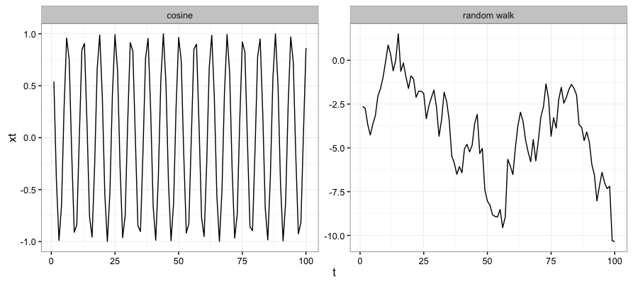
Clearly, I’m still pretty green in this area but it is encouraging that the ‘simple’ time-series ($x_{t}=cos(t)$) has low permutation entropy, indicating less relative complexity than the random walk series.

Some Final Thoughts

A much more experienced time-series analyst in the reading group pointed out that for a handful of time-series that we generated in our group meeting, the Weighted Permutation Entropy had no notable relationship to the maximum Lyapanov Exponent….I don’t spend a lot of time with chaotic dynamics so I’m not all that confident in my understanding of Lyapanov Exponents but this divergence was generally viewed as unsettling.
The abstract of the paper in question hinted that one implication of this line of inquiry (‘model-free quantification of predictability’) was that one could make some inferences about what class of time-series model was likely to yeild the best predictions for time-series exhibiting different “complexities.” If the authors did indeed make some commentary on this subject, they managed to hide it quite well. I read the paper 3 times and didn’t pick up much in the way of evaluating potential for different time-series models to perform in different “complexity” paradigms.
A lot of the stuff in the paper was pretty new to me. My experience with Quantitative Ecology and Mathematical Biology is that sometimes things sound new and exciting to me because they use different words for things that I actually find old and boring…and sometimes things sound new and exciting because Ecologists and Biologists are grappling with problems that have differnt features, constraints, or dimensions than problems typically considered in the Social Sciences…I probably need to read a few more papers in the ‘Complexity Theory’ strand of literature to know where this stuff falls.

Written on November 2, 2016