Initial thoughts on genetic programming

I’ve been casually reading papers on Genetic Programming and Symbolic Regression for a little over a week now so I figured it was high time I stopped thinking about GP and started trying to DO a GP.

What I’ve taken from the stuff I’ve read so far that I thought was really cool is the idea of trying to uncover the underlying structure of data from nothing more than the data itself. There are all sorts of cool applications of GP that I’ve seen but the things that are most relevant to the types of stuff I work on are:

making good predictions from data and
trying to answer questions about the structure of a data generating process in a model-free environment (I’ll talk more about what this means).

PLEASE do not mistake the fact that I’ve written this shit down and posted it on the interweb for expertise. This is basically a lab book for my first attempts at understanding GP/Symbolic Regression. If you want to learn along with me, read on. I think I’ve figured a lot of things out…but there’s undoubtedly a lot I haven’t figured out.

Executive Summary

Genetic programming/symbolic regression is pretty easy to understand conceptually (high level) but really hard (both programmatically and mathematically) to do well.
There is off-the-shelf code available for R, Python, and Matlab users to do simple applications. Doing more sophisticated things like adding penalties for complexity (a simplier solution is better than a complicated one), imposing sensible constraints on the system, forcing the algorithm to consider coupled dynamic systems rather than just univariate problems will probably require a roll-your-own situation…or at least involve picking apart existing code and modifying it.
Especially for some simple functions (sin(x), x^2+x+1) it is REALLY cool to watch a GP evolve programs that recover the target structure from nothing more than a bunch of data points generated from the target functions.
In my opinion, the potential applications of this technique for testing some tride-and-true theoretical restrictions in Ecology and Economics is really exciting.
There are a lot of existing prediction type applications of GP out there. GP evolves programs that can make really good predictions about a range of things…but I’m less excited about this because we already have so many good ensemble Machine Learning predictors (Random Forests, Boltzman Machines, NN, etc, etc)…it’s hard for me to get worked up over ANOTHER awesome ML ensemble learner just for prediction sake.

The Readings

Section 1: Two Motivating Examples:

This shit right here is all about modeling philosophy and has no practical implications for actually doing GP. I highly recommend at best skimming it and possibly skipping it altogether unless you want to engage in some serious feet-on-the-desk, pie-in-the-sky pontification.

Farm Labor and Irrigation Water Supply

Suppose I’m interested in something like the impact of large federally subsidized irrigation water projects (and the water they deliver) on agricultural labor (jobs) in California’s Central Valley….sorry for shamelessly plugging one of my papers. One way to proceed is to specify a labor demand equation which is a function of available irrigation water and fit that equation to observed data. The way this is usually done goes something like this:

Define a profit function axiomatically for a producer facing:

output prices for m outputs $p_{i}$
input prices for k inputs $p_{i}$
total fixed amount of water available, $W$
other fixed inputs, $x$

\[\pi(p,r,W,x)=max_{w_{1},...w_{m}}\sum_{j}^{m}\pi_{j}(p_{j},r,w_{j},x):\sum_{j}^{m}w_{j}=W\]

where the individual $p_{j}$ are crop specific profit functions.

This profit function can be written as,

\[\pi(p,r,W,x)=\sum_{j}^{m}\pi_{j}(p_{j},r,w_{j}^*(p,r,W,x),x)\]

Since we don’t know a priori what functional form the profit function should take, we generally use a form from a class of functions called flexible functional forms…so named because they have enough parameters and enough curvature to offer a good 2nd order Taylor series approximation to an arbitrary function. A popular flexible functional form for profits is the normalized quadratic. The normalized quadratic parameterizes the above axiomatic definition of profits as follows:

\[\Pi(p,r,W,x)=a + B \tilde{P} + 0.5 P'C \tilde{P}\]

the quantities, [a,B,C] are parameters and the notation,

\[\tilde{P}=\tilde{p},\tilde{r},w,x\]

denotes that these quantities have been normalized by one of the outputs or inputs.

The functional response of labor to water is estimated by applying Hotelling’s Rule which says that the first derivatives of the profit function with respect to output prices yield the optimal output supply equations and the first derivatives of the profit function with respect to input prices gives the optimal input demand equations. Applying this rule we get a system of m (number of outputs) + k-1 (number of inputs):

\[\frac{d \pi}{dp_{j}} = y_{j}*\] \[\frac{d \pi}{dr_{j}} = x_{j}*\]

The functional response of agricultural labor demand to available fixed annual quantity of irrigation water will be reflected in the derivative of the profit function with respect to the input price of labor $r_{l}$.

Note that the key highlevel steps here were:

Define a profit function, and
Choose a form that has flexible properties

If we were interested in testing the sensativity of our results to the assumed function form of the profit function we could test out several other functional forms (Translog and Cobb-Douglas are other popular choices).

However, using this approach, at the end of the day, we’re not really testing for the TRUE underlying structure of the system….we’re really just testing whether a system derived from a normalized quadratic, translog, or cobb-douglas functional form fits the data better.

Example 2: Price Dynamics

An alternative to highly structural modeling like fitting data to models derived from Economic Theory (see Example 1) is the totally theory-agnostic approach of Machine Learning. Suppose we want predict coffee prices. We have time series data on coffee prices ($c_{t}$), other commodity prices like cocoa ($cc_{t}$), cotton ($co_{t}$), and a bunch of maybe relevant macro economic time series…like maybe GDP per capita of major coffee consuming nations…call these $Z$ for right now.

If we just want to predict the price series ($c_{t}$) without the burden of specifying a complete structural model that would require us to hypothesize, among other things, what series drive what other series, we could use something really flexible like a Neural Network. Neural Networks work by basically putting a bunch of things in a box that you think might predict coffee prices (coffee prices last period, coffee prices two periods ago, etc, cotton prices, cotton prices two periods ago, Malaysian GDP, Canadian GDP per capita, artic sea ice, whatever). Once all the stuff is in the box, the things get combined in all kinds of ways until the best predictions are generated.

A typical Neural Network looks somethign like this.

Neural Networks can produce really good prediction but they don’t yeild any insight about structure. They can’t really tell you if Artic Sea Ice is a good predictor of coffee price and, even if it could, it doesn’t attach a weight or an empirical impact to that driver. If you look at diagram linked to above, all three inputs map to all three ‘hidden layers’ which might then pass through another ‘hidden layer’ and get further distorted before generating output. Simply stated, there is no way to infer a causal relationship between Artic Sea Ice, Cocoa Price, and Coffee Price from a Neural Network.

An old professor of mine was working of ways of circumventing the normal tradeoff between assumed structure and letting the data speak:

Haigh and Bessler, Causality and Price Discovery: An Application of Directed Acyclic Graphs

Basically, they use Directed Acyclic Graphs to infer what series drive other series. Then they use very flexible estimation techniques like Vector Autoregression to quantify those links.

Recap

In the first example I was really interested in the structure of the data generating process and, by extension, the underlying coupled dynamics of labor and water. In the second example, I was not interested in structure at all…I just wanted good predictions.

GP, I think, provides a way to bridge these two worlds. Upon successful completion of a GP, what I’m going to get (I think) is a symbolic structural representation of the system that best fits my data….but I’m going to get it in a way that didn’t need to impose any a prior constraints on what the structure of the system SHOULD be.

What I really like about GP (so far) is that it adopts the model-free ethos of things Neural Networks but instead of saying, “the structure isn’t really important”, it says, “let me learn the structure from the data.”

Section 2: Genetic Programming in (mostly) words

First order of business is nomenclature: the ‘programs’ that I’m about to talk about here are what most of us would think about as functions or equation. They will be things like,

\[x+y\]

\[sin(x) * cos(y)\]

In Genetic Programming the programs don’t have to be functions. I’ve seen a GP application where the algorithm was used to build a circuit…in that case the ‘program’ was a combination of hardware needed for the circuit…In this case the ‘programs’ will all be functions and (if you’re not already down with GP) it’s going to feel a little funky to hear continually refer to shit like $x+1$ as a program but I want to stop putting quotes around program so just know that by program here I’m talking about the function generated by combining function operators and terminal operators.

Part 1: Setting Up the GP

The conceptual backbone of Genetic Programming and, relatedly, symbolic regression, is that you have some building blocks…if you are trying to recover a structural equation or system of equations that generated some data than the basic building blocks are:

function set: +, -, *, %, sin, cosine, exp,
terminal set: this is the stuff that will be manipulated by the items in the function set. These are things like: variables in the model: x, y, z AND coefficients or constants of the model: 0, 3.5,

The terminal set can also include 0-arity functions like rand(), go_left, etc….but I don’t want to worry about those right now.

To form the initial population, we randomly sample the function set and terminal set and combine these randomly selected elements. The ‘program’ resulting from randomly sampling the function set and terminal set can be displayed as a tree or heirarchy (it actually took me about a half hour to wrap my head around this visual presentation…during that time I was convinced that there was a better way to represent the ‘program’. I tried many alternative visuals but I really think that, once you get used to looking at programs this way, it is the easiest and best way to represent them). Let’s take a quick example,

Suppose I have the function set F = {+,-,*,%} and the terminal set, TS={x,sample(seq(from=-1,to=1,by=0.1),1)}…this means the terminal set can either be x or a randomly sampled number from -1 to 1.

# 1. Assuming the root node is always a function operator I first sample from the function set

sample(F,1)
> 1 


# 2. The next node can be another function operator or an item from the terminal set so I sample these two

sample(c(F,TS),1)
> 'TS'

# since I got back 'TS' for terminal set I now sample the terminal set for a value:

sample(TS,1)
> x

# 3. Now I sample the list=(F,TS) again because my tree depth is set to 2 which means the root node in the population will have two nodes

sample(c(F,TS),1)
>F

# 4. I got the result 'F' for function set so I now sample the function set for the specific operator:

sample(F,1)
> *

# 5. Since I've defined the tree depth to be 2 the children of this node must both be from the terminal set...if the tree depth were #increased we could continue
#iteratively sampling from the function set and terminal set

sample(TS,2)
> x,5

At this point we have everything we need to represent our ‘program’:

our program evaluates to f(x)=x+5x=6x

#—————————————————————————–

Now let’s imagine that we repeat steps 1:5 many times and create a population of programs. Call this Generation 0. For concreteness let’s assume I repeated steps 1:5 a few more times and got three more programs for my initial population. My initial population consists of 4 programs

         +
       / \
     x   *
         /\ 
        x 5

        -
       / \
     1   +
         /\ 
        2 x
 
        *
       / \
     +   *
     /\    /\ 
   -1 x     x 5
 

        +
       / \
     *   1
    /\    
   x 1    

Part 2: Evolving the Population

The next step in the Genetic Program is creating a new generation of programs from the Generation 0. For this we need to introduce the notion of fitness because we will want to select programs for the next generation based, at least in part, on their fitness.

For the time being let’s suppose we have a target function and our goal is to see if, given data generated by our target function, we can recover a really good approximation….or even better recover the symbolic representation of the function.

Let’s assume that the target function is sin(x) and the range over which we want to evaluate it is -pi:pi…so our data are

 [1] -1.224606e-16 -9.983342e-02 -1.986693e-01 -2.955202e-01 -3.894183e-01 -4.794255e-01 -5.646425e-01 -6.442177e-01
 [9] -7.173561e-01 -7.833269e-01 -8.414710e-01 -8.912074e-01 -9.320391e-01 -9.635582e-01 -9.854497e-01 -9.974950e-01
[17] -9.995736e-01 -9.916648e-01 -9.738476e-01 -9.463001e-01 -9.092974e-01 -8.632094e-01 -8.084964e-01 -7.457052e-01
[25] -6.754632e-01 -5.984721e-01 -5.155014e-01 -4.273799e-01 -3.349882e-01 -2.392493e-01 -1.411200e-01 -4.158066e-02
[33]  5.837414e-02  1.577457e-01  2.555411e-01  3.507832e-01  4.425204e-01  5.298361e-01  6.118579e-01  6.877662e-01
[41]  7.568025e-01  8.182771e-01  8.715758e-01  9.161659e-01  9.516021e-01  9.775301e-01  9.936910e-01  9.999233e-01
[49]  9.961646e-01  9.824526e-01  9.589243e-01  9.258147e-01  8.834547e-01  8.322674e-01  7.727645e-01  7.055403e-01
[57]  6.312666e-01  5.506855e-01  4.646022e-01  3.738767e-01  2.794155e-01  1.821625e-01  8.308940e-02

In general the fitness function can really be any error minimizing function (with penalty for non-parismony or whatever) so I’m going to use sum of squared errors as my fitness function…the smaller the sum of squared error is the better the program is and the better chance that program will have of persisting to the next generation.

\[SSE = \sum_{i} sin(x_{i})-f(x_{i})\]

The sum of squared errors for the four programs above are:

SSE=(6781, 182, 38211.05, 171)

Next we need to decided how our programs will evolve from one generation to the next. There are other evolutionary operators but to keep this relatively simple I’m going to use only reproduction, mutation, and cross-over. The mechanics of each will be clear as we proceed.

First I’m going to sample from the list of possible evoluationary operators but I’m going to sample with probability weights: Poli et al. suggest using 25% reproduction, 25% for mutation and 50% for cross-over:

sample(c('reproduction','mutation','cross-over'),4,replace=T,prob=c(0.5,0.25,0.25))
> reproduction, mutation, cross-over,reproduction

Part 2A: Reproduction

This is the simplest of the operators because it just move a program from one generation to the next. In practice, now that we sampled the space of evolutionary operators and got the operator ‘reproduction’ we want to sample the program population space to see which program from Generation 0 will get reproduced.

When we sample the program population we want to use a weighted sampling scheme because we want programs with higher fitness to have a higer probability of being select. Here, because I only have a population size of 4 I’m going to use a simple rule that says the program with the best fitness has a 50% of being selected, the next best program has a 30% chance, the 3rd best has a 15% chance and the worst one has a 5% chance.

sample(c(1:4),1,prob=c(0.15,.3,0.05,0.5))
> 2

This means that our 2nd function from Generation 0 moves into the population for Generation 1.

Part 2B: Mutation

With mutation what happens is that we generate an entirely new program using the same program generator that we used for the initial population. Then we again randomly sample a program from Generation 0 to be mutated. Once we have the program to be mutated and the new program we randomly sample a node in Generation 0 program to be the location of mutation and we swap that node with a randomly selected node from the new program:

First we randomly sample the population of Generation 0 to find the program that will be mutated:

sample(c(1:4),1,prob=c(0.15,0.3,0.05,0.5))
> 2

Next we run the program generator and get the new program:

    -
   / \
  x   %
     / \
    x   1

Next we randomly sample the node from the population program to be the site of mutation and the node from the new program that provides the mutation

sample(c(1:5),2,replace=T)
> 3
> 4

Replacing the 3rd node of the 2nd program in Generation 0 with the 4th node of our new program gives us:

   -
  / \ 
1    x   

Part 2C: Cross-Over

Cross-over occurs when two existing programs swap nodes. When cross-over happens we randomly select two programs from the previous generation, then we randomly select nodes (much like in mutation) that will be the site of cross-over and we swap those nodes. Just like in other operation we want there to be a higher probability of breeding two programs with superior fitness so we, again, use the weighted sampling scheme to select two program from the previous generation to breed:

sample(c(1:4),2,replace=T,prob=c(0.15,0.3,0.05,0.5)) 
> 2
> 4

Next, we randomly select nodes to be the site of cross-over:

sample(c(1:5),2,replace=T)
> 4
> 2

So here we swap node 4 in program 2 from last generation with node 2 in program 4 from last generation:

Part 2D: Reproduction…again

Let’s make this quick. Sample another program from the Gen 0 population program to reproduce:

sample(c(1:4),1,prob=c(0.15,0.3,0.05,0.5)) 
> 4

Generation 1:

So Generation 1 looks like this:

Next Steps

From here just

calculate the fitness of the four programs in Generation 1
use fitness to establish sampling weights to use in the selection of program for next generation
repeat the steps we followed up to this point until you reach some convergence criteria or iteration criteria.

Section 3: An Example By Hand

So I got to a point where I thought I had the basic idea but I needed to try it to see if I really understood the mechanics. So I tried to solve a simple problem by hand - something in between pseudo-code and a full roll-your-own implementation.

WARNING: this is kinda dumb and a little tedious…I suggests reading through the first couple generations to see visually what happens but there is no real reason to go beyond that.

A Field Guide To Genetic Programming by Poli et al. has a sample problem:

given the target function:

$x^2+x+1$ defined over the values [-1,-0.9,-0.8,…0.8,0.9,1] can a GP learn the function from data…or least learn a really good approximation to it?

Here I’m going to use the same basic experiment parameters they used. Namely:

A population size of 4
The function set includes only [+,-,%,*]
The terminal set includes x and a constant randomly chose from the interval [-5,5]
From one generation to the next the probability of subtree cross-over is 50%, the probability of mutation is 25% and the probability of reproduction is 25%
Maximum tree depth of the initial population is 2
The fitness function is the sum of squared errors
This assumption is not in Poli et al. but I define the sampling probabilities from one generation to the next to be .5 for the most fit program of the previous generation, .3 for the 2nd most fit, .15 for the 3rd most fit, and 0.05 for the least fit.

NOTE: this type of algorithm, similar to MCMC, involves a lot of random sampling so the code I’m posting here is mostly illustrative. I’ve included actual results as comments in the code so you can follow what values were obtained and what steps were taken as a result.

library(cwhmisc)

fn.set <- c("+","-","div.prot","*")
term.set <- c("x","samp")

#---------------------------------------------------
#program generating function
prog.gen <- function(nprog){
prog.list <- list()

for(i in 1:nprog){
node1 <- NA
node2A <- NA
node2B <- NA
termAA <- NA
termAB <- NA
termBA <- NA
termBB <- NA

node1 <- sample(fn.set,1)

node2A.pop <- sample(c("fn.set","term.set"),1)

if(node2A.pop=='fn.set'){
  node2A <- sample(fn.set,1)
  #if node 2A is from the function set then we know the next nodes must
  # be from the terminal set
  termAA <- sample(term.set,1)
  if(termAA=='samp'){termAA=sample(c(-5:5),1)}
  termAB <- sample(term.set,1)
  if(termAB=='samp'){termAB=sample(c(-5:5),1)}
}else{
  node2A=sample(term.set,1)
  if(node2A=='samp'){node2A=sample(c(-5:5),1)}
}

node2B.pop <- sample(c("fn.set","term.set"),1)

if(node2B.pop=='fn.set'){
  node2B <- sample(fn.set,1)
  termBA <- sample(term.set,1)
  if(termBA=='samp'){termBA=sample(c(-5:5),1)}
  termBB <- sample(term.set,1)
  if(termBB=='samp'){termBB=sample(c(-5:5),1)}
}else{
  node2B=sample(term.set,1)
  if(node2B=='samp'){node2B=sample(c(-5:5),1)}
}

#now organize the results as a list tree for visual effects
p <- list(node1,c(node2A,node2B),c(termAA,termAB,termBA,termBB))
prog.list[[i]] <- p
}
return(prog.list)
}
#-----------------------------------------------------


#set up the target function
targ.fun <- function(z){(z*z)+z+1}

#set up the values of the interval over which candidate programs will be evaluated
fit.vals <- seq(-1,1,by=0.1)

#I'm just going to change fit values so I don't have to worry about 
# protected division
fit.vals[which(fit.vals==0)] <- 0.001

#evaluate the target function at the values determined above
fit.targ<-unlist(lapply(fit.vals,FUN=targ.fun))

#instead of randomly generating the initial population using the prog.gen() function, I'm #going to start with the same initial population as Poli et al. do in Section 4.
fn1 <- function(x){eval(parse(text="x+1"))}
fn2 <- function(x){eval(parse(text="(x*x)+1"))}
fn3 <- function(x){eval(parse(text="return(2)"))}
fn4 <- function(x){eval(parse(text="x"))}

#write a function to evaluate fitness of any program....sum of squared errors
fitness <- function(prog){
  fit.prog <- unlist(lapply(fit.vals,FUN=prog))
  fit <- sum((fit.targ - fit.prog)^2)
  return(fit)
}



program.fitness <- unlist(lapply(list(fn1,fn2,fn3,fn4),fitness))
> program.fitness
[1]  5.066600  7.700001 18.364599 41.466602

#set up sampling probabilities
probs <- c(.5,.3,.15,.05)

#get ranks
ranks <- rank(program.fitness)

#set up sampling weights
probs.eval <- probs[ranks]

#sample 4 times from the list of programs above but weight the sampling by fitness
sample(1:4,4,prob=probs.eval)
[1] 1 1 1 4
#result = 1,1,1,4

#now for each program selected to make it through probabilistically decide if it 
# should be reproduced, crossed-over, or mutated
sample(c('reproduction','cross-over','mutation'),4,replace=T,prob=c(.5,.25,.25))

[1] reproduction, mutation, reproduction, mutation

Things to note from this set up of Generation 0:

the function $x+1$ has the best fitness (5.066)
the fittest program was selected to persist to the next generation 3 out of 4 times
the evolutionary operations applied to the selected programs will be reproduction, mutation, reproduction, mutation

OK, on to Generation 1:

#Generation 1 Program 1:

#---------------------------------------------------------------------
#the first program gets reproduced so it's the same as it was last time
fn1.1 <- function(x){eval(parse(text="x+1"))}
#---------------------------------------------------------------------

The second program selected from Generation 0(which is also program 1 btw) gets mutated… for mutation we need to do a couple things:

generate a new program
randomly sample a node in the new program and randomly sample a node in the existing program.
swap the randomly sampled node form the existing program with the randomly sampled node from the new program

#--------------------------------------------------------------------

#generate a new program
new.prog <- prog.gen(nprog=1)
new.prog
[[1]]
[[1]][[1]]
[1] "*"

[[1]][[2]]
[1] "4" "%"

[[1]][[3]]
[1] NA  NA  "-3" "0"

#btw in tree structure this is 

#         *
#       /  |
#      4   %
#         / |
#       -3  0

# which evaluates to f(x)=4*1

#next we pick which node in the existing program gets mutated
sample(c(1:3),1)
[1] 2

# Now randomly sample a node from the new program

sample(c(1:3),1)
[1] 1

#in this case I get 1 so I'm going to swap this whole program in 

#so the 2nd node from our first program gets replaced with our entire new program, #creating

#     -
#    / \     
#   *   0
#   /\
#  4  %
#     /\
#    -3 0

fn2.1 <- function(x){eval(parse(text="return(4)"))}


#--------------------------------------------------------------------

So the second program in the new Generation is a mutation of program 1 from Generation 0 which basically evaluates to a constant.

The third program selected for the 1st generation is again x+1 and the third random sample from our (reproduction,mutation,cross-over) menu was reproduction so this function again just persists to the next generation:

#--------------------------------------------------------------------

fn3.1 <- function(x){eval(parse(text="x+1"))}

#--------------------------------------------------------------------

The final program in Generation 1 is program number 3 from Generation 0 and the chosen operation is mutation …so the program f(x)=x gets mutated

#--------------------------------------------------------------------

new.prog <- prog.gen(nprog=1)
new.prog
[[1]]
[[1]][[1]]
[1] "-"

[[1]][[2]]
[1] "5" "+"

[[1]][[3]]
[1] NA  NA  "x" "x"


#generate a new program and pick a node in that program
# the new program generated was 5-(x+x)

#sample the new program...which has 5 nodes
sample(c(1:5),1)
[1] 3

#we get the result 3 corresponding to the node 

#            +
#          /  \
#         x   x

#the original function evaluated to just x...but the tree structure was a bit more complicated:

#             *
#            / \
#           x   -
#              / \
#             -1  -2

# so the original had 5 nodes. we need to sample again to find out which node get mutated
sample(c(1:5),1)
[1] 2
#the result returned was 2 so the new function is:

#            *
#           / \
#          +  -
#        / \  / \
#      x   x -1  -2


fn4.1 <- function(x){eval(parse(text="(x+x)*(1)"))}
  
#--------------------------------------------------------------------

At this point we have the population of programs for Generation 1. The next step is to evaluate their fitness and sample from that population to get the programs that will persist to the next generation:

#--------------------------------------------------------------------
#Now we evaluate fitness 

#evaluate fitness
program.fitness <- unlist(lapply(list(fn1.1,fn2.1,fn3.1,fn4.1),fitness))
program.fitness
[1] 5.066 155.56 5.066 49.1646

probs <- c(.5,.3,.15,.05)

ranks <- rank(program.fitness)

probs.eval <- probs[ranks]
#--------------------------------------------------------------------

In this case, the best fitness is unchanged from the last generation because although the two mutation operators produced less fit programs, the fittest program from Generation 0 was chosen to reproduce…so the average fitness of the population has definitely gotten worse but the ‘best fitness’ is unchanged.

So now we need to sample the programs from Generation 1 to persist to Generation 2 and the evoluationary operators that will be applied to these programs.

#--------------------------------------------------------------------
#sample another 4 times from the programs in generation 1 weighting by the sampling by #fitness
# in this case we have a tie and I'm not really sure what to do about that
# so I'm just going to change the probability weights by hand
sample(1:4,4,replace=T,prob=c(.4,0.05,0.4,0.15))
[1] 3 1 3 1

#now for each program selected to make it through probabilistically decide if it 
# should be reproduced, crossed-over, or mutated
sample(c('reproduction','cross-over','mutation'),4,replace=T,prob=c(.5,.25,.25))
[1] cross-over reproduction reproduction reproduction

This generation will be interesting because we have cross-over which we didn’t experience in the last generation.

Ok, the first Generation 1 program sampled for Generation 2 was Generation 1 program 3 and the operator was cross-over. With cross-over we need to sample the previous generation again to find which program will contribute to the cross-over. Again, it’s important to use the weighted sampling scheme…that way the fitter programs from last Generation have a higher probability of being selected to breed with the current program.

#sample a program from Generation 1...other than program 3...maybe it's kosher to breed a # program with itself I don't know. 
sample(c(1,2,4),1)
[1] 1

#now determine which node in the 1st program gets crossed and which
# node in the second program gets crossed

sample(c(1:5),1)
[1] 4
sample(c(1:5),1)
[1] 4

#so we are swapping out the 4th node in Generation 1 Program 3 for the 4th node in #Generation 1 Program 1

# Generation 1 Program 3 was:

#        -
#       / \
#      +   0
#      /\
#     x  1

# Generation 1 Program 1 is actually the same so swapping the 4th node for the 4th node #changes nothing

fn1.2 <- function(x){eval(parse(text="x+1"))}

Interestingly, the next genetic operators are all reproduction and the programs selected from Generation 1 to reproduce are both f(x)=x+1.

Next, we again evaluate fitness for the population and, in this case, all the programs are functionally the same.

program.fitness <- unlist(lapply(list(fn1.1,fn2.1,fn3.1,fn4.1),fitness))
program.fitness
[1]   5.0666 5.0666 5.066 5.066

I found it somewhat encouraging that, although the average fitness of the population last generation got worse, this generation has pretty good fitness.

On to Generation 3.

For Generation 3 we don’t actually need to sample programs from Generation 2 because they are all the same. So we just start by sampling the evolutionary operators.

#we just need to sample the evolutionary operators
sample(c('reproduction','cross-over','mutation'),4,replace=T,prob=c(.5,.25,.25))
[1] mutation mutation mutation mutation

Here we get four instances of mutation which will all apply to the function:

I’m going to move a little faster through this generation since I think everybody is probably getting the hang of how this works by now:

#--------------------------------------------
#mutate program 1

#run the program generator
#         - 
#        / \
#       +   %
#     / \  / \
#    x  0 x  0

#select the node in population program to mutate
sample(c(1:5),1)
[1] 5

#select the node in new program to replace mutated node with
sample(c(1:5),1)
[1] 5

#new program
#         - 
#        / \
#       +   0
#     / \   
#    x  0   

fn1.3 <- function(x){eval(parse(text="x"))} 
#----------------------------------------------------

#----------------------------------------------------
#mutate program 2

#run the program generator
#         % 
#        / \
#       %   x
#     / \   
#    1  4   

#select the node in population program to mutate
sample(c(1:5),1)
[1] 1


#select the node in new program to replace mutated node with
sample(c(1:5),1)
[1] 3


#new program
#         x 


fn2.3 <- function(x){eval(parse(text="x"))} 
#--------------------------------------------------------

#-------------------------------------------------------
#mutate program 3

#run the program generator
#         - 
#        / \
#       -4   *
#           / \  
#          -1 x

#select the node in population program to mutate
sample(c(1:5),1)
[1] 5


#select the node in new program to replace mutated node with
sample(c(1:5),1)
[1] 1

#new program
#         -
#        / \
#       +  0
#      / \
#     x  -
#       / \
#      -4  *
#         / \
#        -1  x

fn3.3 <- function(x){eval(parse(text="x-4+x"))} 
#----------------------------------------------------

#--------------------------------------------------
#mutate program 4

#run the program generator
#         % 
#        / \
#       x   %
#           / \  
#          x   x

#select the node in population program to mutate
sample(c(1:5),1)
[1] 1

#select the node in new program to replace mutated node with
sample(c(1:5),1)
[1] 1

#new program
#         % 
#        / \
#       x   %
#           / \  
#          x   x

fn4.3 <- function(x){eval(parse(text="x"))} 
#----------------------------------------------------------

#------------------------------------------------------
#evaluate fitness for generation 3:
#evaluate fitness
program.fitness <- unlist(lapply(list(fn1.3,fn2.3,fn3.3,fn4.3),fitness))
[1] 41.4666  41.4666 614.7566  41.4666

probs <- c(.5,.3,.15,.05)

ranks <- rank(program.fitness)

probs.eval <- probs[ranks]
#--------------------------------------------------------------------

So you’ll notice that this generation basically returned three different versions of f(x)=x and another function which evaluates to 2(x-2)

A couple of observations:

I actually screwed this up a little in the sense that I meant to use probability weights (0.25,0.5,0.25) for (reproduction, cross-over, mutation) but I actually used probability weights (0.5,0.25,0.25) which oversampled the ‘reproduction’ operator relative to what I meant to do.
I also used a pretty small population size. These two facts together meant that, I was experiencing a lot of redundancy…basically getting a bunch of copies of the same function. In a larger program this would be pretty inefficient.
Efficiency needs to be balanced with diversity. The two programs below both evaluate to x+1. However, there are some good reasons to keep both in the population. The genetic algorithm is non-greedy which means it has an easier time escaping local minima than a greedy search. Part of the non-greedy nature is that genes (nodes), even in less fit programs, always have some probability of wandering off into some other part of the solution space. Simplifying programs that are empirically the same lessens the chances of genes wandering off and forming fitness improving mutations.

   -
  / \
 x   -1

   +
  / \
 x   *
     /\
     x %
      / \
      1  x

Section 4: The Black Box

Now that I’ve done a few generations by hand and I’m confident I have some idea what the Genetic Program is doing, I’m going to try a black box implementation using the ‘rgp’ package in R.

I’m going to try and solve the same problem as last section: recover the function f(x)=x^2+x+1.

library(rgp)

#Basic building blocks
functionSet1 <- functionSet("+","-","*")
inputVariableSet1 <- inputVariableSet("x")
constantFactorySet1 <- constantFactorySet(function() rnorm(1))

#Defining the 'fitness' function
#this part is specific to the evaluation of the function x^2+x+1 
#   over the interval -1:1
interval1 <- seq(from=-1,to=1,by=0.1)
fitnessFunction1 <- function(f)rmse(f(interval1),(interval1*interval1)+interval1+1)

#performing the GP run
set.seed(1)
gpResults1 <- geneticProgramming(functionSet=functionSet1,
                                 inputVariables=inputVariableSet1,
                                 constantSet=constantFactorySet1,
                                 fitnessFunction=fitnessFunction1,
                                 stopCondition=makeTimeStopCondition(2*60))




#plot results....not totally sure how to recover the symbolic expression of the 
# optimal function so I'm doing it by hand here:

gpResults1$population[which.min(gpResults1$fitnessValues)]

fn.opt <- function(x){
  return(0.999621 + (x * x + (x-x*x) + (x-(x+x-x*x))+x))
}

target <- function(x){(x*x)+x+1}

z <- target(interval1)
z.est <- fn.opt(interval1)

ggplot(data.frame(x=interval1,y=z),aes(x=x,y=y)) + geom_line() + 
  geom_line(data=data.frame(x=interval1,y=z.est),aes(x=x,y=y),color="red") + theme_bw()

Recovering Structure

If we look at the output from the genetic program we can access the symbolic representation of the solution it found:

gpResults1$population[which.min(gpResults1$fitnessValues)]
[[1]]
function (x) 
0.99962153075706 + (x * x + (x - x * x) + (x - (x + x - x * x)) + 
    x)

Astute readers will notice that the GP has recovered the target function almost exactly. After some algebraic manipulation we can see that the function it found is,

\[0.9962 + x^2 + x\]

So that’s REALLY cool.

Redundancy

We can get a look at the programs that were in the population on the last iteration by extracting the list object ‘population.’ If we do that we see something rather interesting: at the termination of evolution we end up with a lot of copies of the same function…the fitness maximizing function.

> gpResults1$population
[[1]]
function (x) 
x

[[2]]
function (x) 
0.99962153075706 + (x + (x - (x + x - x * x)) + x)

[[3]]
function (x) 
1.3667619084903 + x

[[4]]
function (x) 
0.99962153075706 + (x * x + (x - x * x) + (x - (x + x - x * x)) + 
    x)

[[5]]
function (x) 
x * x + (0.99962153075706 + x)

[[6]]
function (x) 
x

[[7]]
function (x) 
0.99962153075706 + (x * x + (x - x * x) + (x - (x + x - x * x)) + 
    x)

[[8]]
function (x) 
x

[[9]]
function (x) 
x

[[10]]
function (x) 
x

[[11]]
function (x) 
x

[[12]]
function (x) 
x

[[13]]
function (x) 
1.3667619084903 + x

[[14]]
function (x) 
x * x + (0.99962153075706 + x)

[[15]]
function (x) 
x

[[16]]
function (x) 
x

[[17]]
function (x) 
x

[[18]]
function (x) 
x

[[19]]
function (x) 
x

[[20]]
function (x) 
x

[[21]]
function (x) 
x

[[22]]
function (x) 
0.99962153075706 + (x * x + (x - x * x) + (x - (x + x - x * x)) + 
    x)

In fact, to take this a step further. If we were to rank all the programs in the population by fitness we would see that the top 10 programs are all identical:

\[0.9962153075706 + (x * x + (x - x * x) + (x - (x + x - x * x)) + x)\]

Greedy v. non-greedy

In my handwritten example from Section 3 we noticed that after a couple generations the fitness was actually getting worse. In my experience with the R package this tends to happen a lot in the early stages of evolution of a GP. The conceptual reason why this is good is similar to some dynamic programming algorithms that get worse before they get better: when you’re dealing with a complicated non-linear function you kinda want your algorithm to cast a wide net…you want it to wander around the parameter space/state space/solution space for a while to avoid getting caught in a steepest decent right to a local minima.

In this case the probabilistic nature of evolution ensures the algorithm will tend to wander around the solution space for a while before begining to coverge to ‘optimal’ program stuctures.

Another interesting implication of this is that, without any modifications, the R package will just keep evolving until you tell it to stop. Basically, all the problems I’ve run so far have been characterized by:

A lot time initially spent around the same fitness values or fitness values that initially get worse (the real life explanation for this is: evolution happens slow)
A threshold iteration where fitness gets really good really fast.
A lot of time spent trying to ‘tweek’ a really good solution. Now, I’ll bet anything that you could control this pretty easily by setting some convergence tolerance and penalizing programs that are adding more complexity than the residual variation explained by that complexity. I kind of like that the program keeps looking and keeps trying to make marginal improvements because I’m not interested in GP for function approximation or prediction. If all you want is approximation or prediction and the target function is f(x)=sin(x) you don’t need to let a program run very long…there are lots of equations/polynomials that can provide a great fit to data generated from f(x)=sin(x)…but I’m interested in systems where the structure of the data generating process is of primary interest. I already know I can approximate/estimate the data generated from these systems. I don’t want to do that. I want GP to uncover the symbolic representation of these data generating processes. Therefore, I want it to run beyond the point of just finding really good fits.

The GP I ran on the function f(x)=x^2+x+1 found the target program in under 2 minutes. That seems long to me but I also didn’t test out other limits…so maybe it found the function a lot faster then just spent the rest of the time trying to make some marginal improvement.

Below I’ve copied some of the output that was printed to the console during the GP run because I think it’s informative:

STARTING genetic programming evolution run (Age/Fitness/Complexity Pareto GP search-heuristic) ...
evolution step 100, fitness evaluations: 4950, best fitness: 0.244261, time elapsed: 0.99 seconds
evolution step 200, fitness evaluations: 9950, best fitness: 0.235338, time elapsed: 1.72 seconds
evolution step 300, fitness evaluations: 14950, best fitness: 0.156976, time elapsed: 2.52 seconds
evolution step 400, fitness evaluations: 19950, best fitness: 0.114865, time elapsed: 3.31 seconds
evolution step 500, fitness evaluations: 24950, best fitness: 0.114865, time elapsed: 3.95 seconds
evolution step 600, fitness evaluations: 29950, best fitness: 0.056947, time elapsed: 4.76 seconds
evolution step 700, fitness evaluations: 34950, best fitness: 0.012861, time elapsed: 5.5 seconds
evolution step 800, fitness evaluations: 39950, best fitness: 0.012861, time elapsed: 6.18 seconds
evolution step 900, fitness evaluations: 44950, best fitness: 0.012861, time elapsed: 6.81 seconds
evolution step 1000, fitness evaluations: 49950, best fitness: 0.012861, time elapsed: 7.46 seconds
evolution step 1100, fitness evaluations: 54950, best fitness: 0.012861, time elapsed: 8.31 seconds

evolution step 16200, fitness evaluations: 809950, best fitness: 0.000378, time elapsed: 1 minute, 55.16 seconds
evolution step 16300, fitness evaluations: 814950, best fitness: 0.000378, time elapsed: 1 minute, 55.92 seconds
evolution step 16400, fitness evaluations: 819950, best fitness: 0.000378, time elapsed: 1 minute, 56.68 seconds
evolution step 16500, fitness evaluations: 824950, best fitness: 0.000378, time elapsed: 1 minute, 57.49 seconds
evolution step 16600, fitness evaluations: 829950, best fitness: 0.000378, time elapsed: 1 minute, 58.3 seconds
evolution step 16700, fitness evaluations: 834950, best fitness: 0.000378, time elapsed: 1 minute, 59.09 seconds
evolution step 16800, fitness evaluations: 839950, best fitness: 0.000378, time elapsed: 1 minute, 59.91 seconds
Genetic programming evolution run FINISHED after 16811 evolution steps, 840500 fitness evaluations and 2 minutes, 0 seconds.
> 

Just For Fun

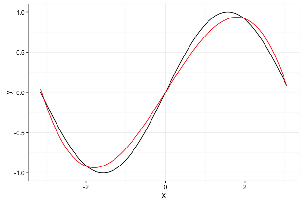
So just for fun I’m going to use the GP package to try and learn the function f(x)=sin(x). This is example that is in the R Vignette for the RGP package. The kicker is that we’re still only going to use the really basic function set [+,-,X]…so basically we’re just going to find the best polynomial approximation to the function f(x)=sin(x).

As seen below…the best polynomial approximation to the sin curve is pretty good over the interval $-\pi$ to $\pi$.

library(rgp)

#Basic building blocks
functionSet1 <- functionSet("+","-","*")
inputVariableSet1 <- inputVariableSet("x")
constantFactorySet1 <- constantFactorySet(function() rnorm(1))

#Defining the 'fitness' function
#this part is specific to the evaluation of the function sin(x) 
#   over the interval -pi:pi
interval1 <- seq(from=-pi,to=pi,by=0.1)

#fitnessFunction1 <- function(f)rmse(f(interval1),(interval1*interval1)+interval1+1)
fitnessFunction1 <- function(f)rmse(f(interval1),sin(interval1))

#performing the GP run
set.seed(1)
gpResults1 <- geneticProgramming(functionSet=functionSet1,
                                 inputVariables=inputVariableSet1,
                                 constantSet=constantFactorySet1,
                                 fitnessFunction=fitnessFunction1,
                                 stopCondition=makeTimeStopCondition(2*60))




#plot results....not totally sure how to recover the symbolic expression of the 
# optimal function so I'm doing it by hand here:

gpResults1$population[which.min(gpResults1$fitnessValues)]


fn.opt <- function(x){
  return(x * -0.080618198828 * (x*x) + x * -0.21904319887 + x)
}

target <- function(x){sin(x)}

z <- target(interval1)
z.est <- fn.opt(interval1)

ggplot(data.frame(x=interval1,y=z),aes(x=x,y=y)) + geom_line() + 
  geom_line(data=data.frame(x=interval1,y=z.est),aes(x=x,y=y),color="red") + theme_bw()

sine wave

Written on January 27, 2017