The empirical section of this post is still a work-in-progress but the data and R scripts are available in my crime repository on GitHub.

Intro/Background

In 1982 Kelling and Wilson published their article in The Atlantic Monthly titled: “Broken Windows: The Police and Neighborhood Safety.” Perhaps because I have followed the academic and public policy discussions surrounding “Broken Windows” policing, I was kind of surprised to hear a segment on NPR today that made it clear to me that there are still a lot of people who think the “Broken Windows” metaphore is associated with time-tested successful policing strategies. I guess I thought everyone basically knew that policing based on the “Broken Windows” hypothesis has been empirically shown to have extrememly questionable/uncertain benefits.

A slightly more general grip related to this post on “Broken Windows” policing: In my opinion too many people crave simplicity with respect to policy prescriptions. Too many people are romantically involved with the notion that “the right answer is usually the simplest one.” Our world is complex, interactions are non-linear, people’s behaviors are nuanced and idiosyncratic. I think it’s foolish to assume we can credibly approach complicated problems like public safety and crime with simple, meme-like solutions.

A Quick Bit of Nomenclature and History:

• In 1969 a Stanford psychologist, Phillip Zimbardo, arranged to have two cars without license plates abandoned on the street. One in Palo Alto, CA and another in The Bronx, NY. He observed that the car abandoned in the Bronx was basically ripped apart and sold for parts within 10 minutes of being abandoned. The car in Palo Alto sat untouched for about a week until Zimbardo himself broke a window. After that, the car was far game and got ransacked pretty quickly. He took this as evidence that disorder invites disorder.

• “Broken Windows” is a theory of policing that seems to have originated with Kelling and Wilson - and has its intellectual roots in the Zimbardo experiment - that says that policing low level offense vigorously reduced more serious crime…“Broken Windows” says if you turn a blind eye to vandalism, graffiti, and various other low level offenses you create an environment that invites more serious crime but if you prosecute these low level offense vigorously you can keep serious crime at bay.

• In 1990 Bill Bratton was promoted to Chief of New York City’s Transit Authority. He implemented what is thought to be one of the earliest and most significant policing strategies based on the “Broken Windows” hypothesis. He energetically prosecuted fare-dodging, graffitti, and other low level public transit related offenses. In 1993 when Rudy Guiliani was elected Mayor, Bill Bratton become the Chief of Police and brought his “Broken Windows” inspired policing strategy to the NYPD. The experience of New York City in the 1980s and 1990s is often used in empirical evaluations of the efficacy of “Broken Windows” policing because of these events.

A Quick Point of Order:

From now on when I used the term “Broken Windows” hypothesis or “Broken Windows” theory I am specifically referring to the ideas that vigorously policing and prosecuting low level crimes can produce declines in more serious crimes. I don’t dispute Zimbrano’s psychological construct that disorder breeds disorder. I do however dispute that this ideas means policing tactics centered on pursuing litterers and vagrants leads to reduction in the murder rate.

Outline

As both of my regular readers know, I like to provide the goals and highlights of every post up-front…that way nobody has to get halfway through a few thousand words before realize that they are not at interested in the topic/analysis at hand.

Some background resources if you want them

I wrote a few primers on empirical analysis of public policy over at The Samuelson Condition

• The Synthetic Control Method
• A Difference in Differences Primer

Here’s What I Plan to Do

• I’ve scanned a large swarth of literature that utilizes data to test the efficacy of “Broken Windows” policing. I’ve also studied in-depth a few papers in this literature that I consider to be particularly reputable (either because they appear in quality journals or because I scanned the methods sections and found them to be reasonably rigorous). I’m going to provide a review of these resources viz-a-viz i) how the analysis is conducted, ii) what data sources are leveraged, and iii) what they say positive or negative about the efficacy of policing strategies based on the “Broken Windows” hypothesis.

• For most of the literature I’m going to review here I’ve tried to ascertain whether the data used is readily available and whether quick replication is possible. In most cases it is not…but there are some easy to access data sources on historical crime rates. In the 2nd part of this post I provide some code for accessing and analyzing publicly available data on crime.

Executive Summary

First: what is my the verdict on the “Broken Windows” hypothesis?

1. I think it was a good idea advanced by two well-meaning researchers looking to solve an important problem (how to keep communities safe with limited law enforement resources)

2. Despite being a good idea at the time it was proposed, I believe that a proponderance of the empirical evidence has shown highly uncertain benefits to policing strategies based on the “Broken Windows” philosophy.

3. The metaphore of “Broken Windows” is really powerful in its simplicity. This is probably why the idea has persisted in the public conciousness despite the fact that data has shown it to be of dubious quality. I’m generally inclined to forgive researchers whose ideas get hi-jacked to satisfy an agenda…In this case however, I don’t think Kelling and Wilson get off that easy. I’ve heard interviews where at least one has basically admitted that elementary data analysis can quickly cast shadows on the “Broken Windows” hypothesis but said that didn’t change his belief that “Broken Windows” was a solid foundation for policing strategies. Look man, I’m a researcher and a scientist too. I have ideas and I try to turn them into something that can be helpful. Sometimes I’m successful and sometimes my ideas are just wrong. People who are willing to cling to an idea in the face of overwhelming evidence that the ideas is bunk are called advocates, not scientists.

4. If we wanted to boil down the empirical challenges with proving or disproving that “Broken Windows” works to its essence, it would probably be this: Generally speaking, in order to implement “Broken Windows” you need to add more cops. Once you start increasing the law enforcement footprint it becomes difficult to untangle the “more cops” effect from the “broken windows” effect. Some people might say that it doesn’t matter and you don’t need to untangle those effects (if crime went down that’s good full stop…it doesn’t matter if it was because there were just more cops or because broken windows policing works). Those people are wrong and they need a stronger understanding of tradeoffs.

It matters for the following reason: If you are a police force with 20 men and you are not using a “Broken Windows” strategy (presumably because you lack the man power) and your force doubles, you have to choose how to employ those extra resources. If broken windows works then you should use those extra men to vigorously prosecute petty crime. But there is an alternative to “Broken Windows” that many like to call “Community Policing.” Rather than spend all your time and energy arresting vandals, this theory goes, police need to be out spending time in the communities they are protecting. Building trust, goodwill, good vibes, etc. “Broken Windows” has been shown to have a social cost in the sense that certain communities (especially ones of color) feel unfairly targeted by “Broken Windows” and learn to distrust and resent cops. If the “Broken Windows” effect is really just a “more cops” effect then there is no reason to risk the social cost associated with broken windows policing…you’re way better off employing “Community Policing” because it gets you the same reduction in violent crime (because the reduction in violent crime is due to more cops not broken windows policing) without the backlash.

Second: what are some high points from my lit review/data exploration?

1. I was a little dismayed at how difficult it was to find a proper difference-in-differences study on this topic. This seems like the perfect set-up for a treatment-control study and couldn’t find one of the quality that I had hoped would be out there. Basically, if we want to know if “Broken Windows” policing works we really need to find (a) a place where it was it was implemented and (b) a place that did not implement “Broken Windows” type policing but that is very much like the place that did.

2. I was a little dismayed at how difficult it was to (a) find out what data authors were using and where it came from and (b) find actual data sources once I thought I understood what data each author was using. My dismay may partially explain #1…that is, maybe there are no good D-i-D studies because there aren’t good time-series data on crime for any areas other than a small number of big metropolitan areas and state-level aggregates…this is a shame. With the attention that this topic has gotten I would hope it would be easier to compare outcomes for NY and - for example - surrounding smaller cities that may police differently.

This is actually a general grievance I have with Economics and Social Science in general. I am an economist but I work in an agency dominated by physical scientists. I can say with extreme confidence that biologists and other ‘hard’ scientist are much more transparent about the data they work with. Too many economists (IMHO) can get away with vagaries like, “we used time-series data on crime in New York obtained from the NYPD” and still get published in good journals. This shit would never fly in the environmental science/ecology literature. When you see a climate change study that uses sea-surface temperature it will almost always be accompanied with a statement in the paper like, “we used the SST-007-monthly-97568 series accessed from the ERDAP server on 11/20/2016. The series can be downloaded from ERDAP with the followign API call….”

1. I was more than a little dismayed at how easy it was for me to find strong empirical evidence that ‘broken windows’ is a broken/useless theory and how many people supporting ‘broken windows’ are still clinging to its value even in the face of overwhelming empirical evidence that it doesn’t work.

2. I’ve had some harsh words for Steve Levitt and Freakonomics in the past. I didn’t love the Levitt analysis from Freakonomics on abortions and crime. I thought it was seriously flawed but it does provide a refreshing wake up call on the ‘broken windows’ discussion. That is, one of Levitt’s explanations for the reduction in the crime rate in the 1990s was that Roe v. Wade legalized abortion in 1970. On it’s face that explanation seems far-fetched and much less intuitive than the ‘broken windows’ explanations. However, ‘broken windows’ has been shown to have no more statistical power to explain the drop in crime in NY in the 1990s than Levitt’s alternative hypothesis. To me what that says is that the ‘broken windows’ crowd has posited an explaination for declining crime rates that is simple and intuitive yet has no more empirical validity than a far-fetched, seemingly rediculous theory about abortion rates. If it takes more than that the finally put the nail in the ‘broken windows’ coffin than I really don’t understand how people evaluate evidence and form opinions.

Methods Overview

Empirical work related to the “Broken Windows” hypothesis comes in a lot of flavors. I contend that most of the literature falls into two basic camps:

1. Regression-based analysis using misdemeanor arrests as a proxy for broken windows policing. These studies generally use murder or some other violent crime as the dependent variable in a regression and include some combination of economic factors, demographic factors, and policing strategy as explanatory variables. Consider the following equation:

Here TEENS controls for population structure (a younger population is generally considered to be a more crime-prone population), COPS controls for size of police force, UNEMP is the unemployment rate and controls for economic factors, and month controls for seasonal factors (maybe crime tends to be higher in the summer).

Generally speaking, if $\rho$ is negative and significant it means that - holding other things constant - increasing misdemeanor arrests (or some other broken windows proxy) tends to significantly decrease incidence of violent crime.

1. Treatment-control type studies. In these studies authors choose a ‘treatment’ area that was known to have implemented some type of broken windows related policing strategy and some ‘control’ area which are (ostensibly) similar to the treatment area but differed in their adoption of broken windows policing. Outcomes compared across the different areas should yield some insight as to whether broken windows policing reduces violent/serious crime.

Part I: A Review of Some “Broken Windows” Literature

There are 4-5 papers I found in the scholarly literature that I felt were sufficiently data driven to warrant inclusion in this post (Note: there are tons of papers on this topic in the law literature. That shit is not really my bag baby…it tends to be really wordy, the papers are really long, and there are no equations. The no equations thing might be a selling point for some people so don’t let me turn you off of the law review lit…just don’t expect me to read it.)

Levitt: Journal of Economic Perspectives

This is probably one of the most compact, concise, and unapologetic rebukes of “Broken Windows” that you’ll find. It was published in the Journal of Economic Perspectives but if you don’t have scholarly journal access a .pdf is available here…It’s called “Understanding why crime fell in the 1990: four factors that explain the decline and six that do not.

I won’t leave you in suspense. The 4 factors that matter, according to Steve Levitt are:

1. Increase in the number of police
2. Rising prison population
3. The receeding crack epidemic
4. Legalization of abortion

The 6 factors that had no influence:

1. The strong economy of the 1990
2. Changing demographics
3. Better policing strategies
4. Gun control laws
5. Concile-and-carry laws - I thought this one was interesting. From Levitt’s paper, The empirical work in support of this hypothesis, however, has proven to be fragile along a number of dimensions (Black and Nagin, 1998; Ludwig, 1998; Duggan, 2001; Ayres and Donohue, 2003). First, allowing concealed weapons should have the greatest impact on crimes that involve face-to-face contact and occur outside the home where the law might affect gun carrying. Robbery is the crime category that most clearly Ž ts this description, yet Ayres and Donohue (2003) demonstrate that empirically the passage of these laws is, if anything, positively related to the robbery rate. More generally, Duggan (2001) Žnds that for crimes that appear to decline with the law change, the declines in crime actually predate the passage of the laws, arguing against a causal impact of the law. Finally, when the original Lott and Mustard (1997) data set is extended forward in time to encompass a large number of additional law enactments, the results disappear (Ayres and Donohue, 2003). Ultimately, there appears to be little basis for believing thatconcealed weapons laws have had an appreciable impact on crime.
6. Increased use of capital punishment

This Levitt paper doesn’t offer a lot of primary analysis, it’s mostly a review of other studies. It’s a very good review and you should read it. In his criticism of the myth that broken windows policing lowered crime in the 1990s Levitt makes a few points that I enjoyed:

• Several quasi-randomized studies discussed in Wilson, 1995 failed to provide convincing evidence that broken windows policing lowered crime.
• Much has been made of the New York experience because crime dropped so precipitously there during the 1990s. Levitt points out that none of the studies using New York as an example have clearly articulated when the “broken windows” era of policing was supposed to have started. Since violent crimes began a rather rapid decline in New York somewhere around 1989/1990 it’s kind of important – if you think broken windows was the reason – to decide when broken windows started.
• Levitt also points out that a paper by Corman and Mocan (it was an NBER working paper when the Levitt paper was published by has since been published in the Journal of Law and Economics did not reliably control for the fact that the end of the crack epidemic basically coincided with the huge drop in violent crime in NY. This is perhaps a small quibble…however, the evidence in favor of efficacy of broken windows from Corman and Mocan (2005) was rather weak to start with (they found a significant effect for robbery and motor vehicle theft but no effect for murder or other violent crimes). So a small quibble about control for the crack epidemic takes on a bit more weight when the results were a little tenuous in the first place.

Corman and Mocan (2005)

There isn’t much I need to say about this paper that wasn’t covered in the Levitt paper…but since it’s an oft-cited paper in a solid journal that seems to support the broken windows paradigm, I should at least give a quick summation: The authors use monthly data (1974-1999) from New York City. The estimating equation they use is:

$CR_{it}$ is the $i^{th}$ crime in month $t$. Economic conditions are captured by the unemployment rate and the real minimum wage. Prison population and size of police force are included to capture ‘deterant’ type effects. Misdemenor arrests is included to capture the effect of broken windows policing.

I give Corman and Mocan props for being careful with the time-series properties of the data. This is something that I think the softer social science literature on “broken windows” ignores…and that ignorance compromises the validity of results, IMO. Corman and Mocan run the appropriate battery of time-series tests (tests for unit roots, tests for stationarity, test for integration order among variables), which I very much appreciated.

Here is something that really troubled me about this paper: If you look at the plots of monthly time series for individual crimes in the paper you’ll notice a few important details:

• Murders in NYC appear to have peaks in Jan 1990 or possibly Jan 1991 and have trending down since then.
• Burglaries have been trending notably down since around Jan 1980
• Felony assault peaked around Jan 1988 or 1989 and dropped month-after-month since then.

A reasonable assumed starting point for broken windows policing in NYC is often considered to be 1993 (Guiliani became mayor and appointed Bratton Chief of Police). But an alternative time-line might put the start of broken windows in 1990 when Bratton was named Chief of the NYC Transit Police. The 1990 start date would coincide with the start of a decline in murders. HOWEVER, murder was one of the crimes for which the “broken windows” coefficient was found to be insignificant. The broken windows coefficient was found to be significant for burglary but burglaries in NYC have been in a virtual free-fall since 1980, ten years before the earliest possible start of broken windows policing. Felony assault declines don’t miss the “broken windows” era by very much…HOWEVER, the broken windows coefficient was found to be insignificant in the felony assault equation.

Another thing that troubled me about this paper was the presentation of results. They basically ran like 8 regressions and found a significant “broken windows” effect in 2 of them. They hold this up as “some” evidence that “broken windows” policing works. I think that’s dishonest. If you had to run 8 regressions equations a bunch of different ways (possibly 40 estimations) just to get 2 significant coefficients, then you didn’t find “some” evidence…you found really weak to probably spurious evidence.

Braga and Bond, 2008

Warning, this is a really long paper. On the spectrum of papers lending empirical support to broken windows and papers demonstrating a lack of empirical support for broken windows I put this somewhere in the middle. I think this paper has probably been held up as evidence that broken windows works but there is a lot of nuance in the paper worth paying attention to. For starters I’ll call your attention to this passage in the conclusion:

These findings suggest that when adopting a policing disorder approach to crime prevention, police departments should work within a problem oriented policing framework and adopt a community coproduction model rather than drift toward a zero tolerance policing model that focuses on a subset of social incivilities, such as drunken people, rowdy teens, and street vagrants, and seeks to remove them from the street via arrest (Taylor, 2001, 2006). Misdemeanor arrests obviously play a noteworthy role in dealing with disorder; however, arrest strategies do not deal directly with physical conditions.

One of the interesting tid-bits in this paper was a finding that improving the physical appearance of a crime hot-spot tends to significantly reduce serious crime. This is broadly consistent with the original Zimbrano “Broken Windows” idea that disorder begets disorder. However, it is pretty different from the Guiliani/Bratton interpretation of “Broken Windows” which says you need to pursue and arrest petty crimes. Basically, Braga and Bond found that cleaning up trash and removing graffiti help curb more serious crime almost as much (and possibly more) than arresting a litterer or vandal.

Keizer, Lindenberg, and Steg, 2008

The Spreading of Disorder by Keizer, Lindenberg, and Steg has also been held up as a win for “Broken Windows.” This one is a little easier for me to dismiss because while it does support the spirit of Zimbrano’s hypothesis , it doesn’t deal in any specific terms with law enforcement interventions.

It does establish that people are more likely to litter if they see litter on the street and more likely to leave a shopping cart in the parking lot if they see a bunch of shopping carts in the parking lot. However, they don’t test whether arresting people for littering curbs littering let alone curbs violent crime.

I’m going to file this one in the ‘NA’ category but I do have a few rant-type sentences for the paper overall:

I think the authors of this study were cagey and sloppy with respect to the social-psychological mechanisms they claim to have informed with this paper. In particular, saying,

1. “people are more likely to litter if they see somebody else littering” and
2. “people are more likely to litter if they see litter about”

are two closely related things with very different implications. In the first case, the individual perceives there is little risk of punishment from littering and so the individual can safely litter. In this case, law enforcement might do pretty well to stay on top of prosecuting litterers…in the second case, if you want less litter, you just need to pick up existing trash more frequently.

It pisses me off that people can get in a journal like Science without being careful about this distinction because I publish in low-level field journals with much lower impact factors than Science and I can tell you with certainty that I would get raked over the coals for not being specific and careful with my study implications.

A few more for the lightening round:

Harcourt, 2006, University of Chicago Law Review

Our analysis provides no empirical evidence to support the view that shifting police towards minor disorder offenses would improve the efficiency of police spending and reduce violent crime

Torres, Apkarian, and Hawdon, 2016, Social Sciences

Abstract

Banishment policies grant police the authority to formally ban individuals from entering public housing and arrest them for trespassing if they violate the ban. Despite its widespread use and the social consequences resulting from it, an empirical evaluation of the effectiveness of banishment has not been performed. Understanding banishment enforcement is an evolution of broken windows policing, this study explores how effective bans are at reducing crime in public housing. We analyze crime data, spanning the years 2001–2012, from six public housing communities and 13 surrounding communities in one southeastern U.S. city. Using Arellano-Bond dynamic panel models, we investigate whether or not issuing bans predicts reductions in property and violent crimes as well as increases in drug and trespass arrests in public housing. We find that this brand of broken windows policing does reduce crime, albeit relatively small reductions and only for property crime, while resulting in an increase in trespass arrests. Given our findings that these policies have only a modest impact on property crime, yet produce relatively larger increases in arrests for minor offenses in communities of color, and ultimately have no significant impact on violent crime, it will be important for police, communities, and policy makers to discuss whether the returns are worth the potential costs.

Some Data Analysis of Our Own

I had hoped to get much further on this and actually try to replicate results from some of the studies I mentioned above. In my quest to do some replication I was primarily stymied by the fact that I could not find time series data on the number of police employed by state or city. This is a pretty key variable in all of the empirical studies and without it I don’t think we can do much here in the way of replication.

What we can do is at least look at some of the statewide and city wide trends to get a feel for how we might use some of these data in the future. As I said, I think data on crime and policing should be easier to find but here is what I did find:

1. Statewide estimates of violent crimes, property crimes, and car theft from 1960 to 2012. I got these from Quandl via the FBI’s Uniform Crime Reporting system. Notably, this data series does not contain arrests for low level misdemeanors which is an important proxy for “broken windows” policing in the empirical studies.

2. Estimates of violent crime, property crime, and car theft for selected major cities from 1985 to 2012. I got these directly through the FBI’s UCR data tool and it was a pain in the ass because I could pull all major crimes for a single city…or all major cities for a single crime variable. But I could not do both…so I had to do a lot of pointing and clicking to download all the cities with populations greater than 500,000.

3. Statewide unemployment rates I got from Quandl, these were pretty easy to get.

4. I did find one source for data on number of police employed. The Bureau of Labor Statistics has a series (NAICS 922120, Police Protection) from the Quarterly Census of Employment and Wages. I had to pull these individually by state which as a pain and several states had a lot of missing values…Also, the time series is only 2005 - 2015 which limits what we can do with these.

5. Finally New York and California both had an Open Cities website where I was able to get crime and arrests for smaller cities. These data included misdemeanors so a bargain-brand replication of the Corman and Mocan study is possible….I added county level population numbers that I go from Quandl.

• California crime stats are here
• New York I got from here

A WARNING:

This section is going to be pretty light. You should look at this for what it represents: I did a lot more work that I had planned on trying to find data that could help us do some of our own analysis on this topic. So basically, I’m giving you all a little head-start on your own “Broken Windows” empirical analysis. There are still some pretty important gaps. In order to do our own version of a Corman and Mocan-type analysis we’ll need to figure out how to get

• population and unemployment numbers at the county level…or
• misdemeanor arrests at the state level

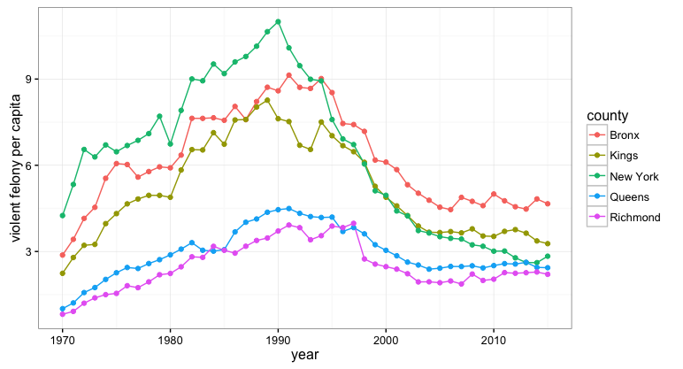
A Quick Look at NYC

So the first thing I want to do here is plot some of the New York City crime data just to make sure the data I pulled has the same broad trends as the ones described in the paper I reviewed above…this is just a quick red-face check to make sure we’re dealing with the ‘right’ data

The population data and crime data for New York are organized at the county level so we will plot each of the 5 counties that encompass New York City (as I understand it each of the 5 Boroughs are in their own county).

# Let's look at just the New York Data because they have a pretty nice data set 
# on crime across all areas of the state

ny.crime <- read.csv("data/arrests_NY.txt")

names(ny.crime) <- c('county','year','total','felony_total','drug_felony','violent_felony','dwi_felony','other_felony',
                     'mis_total','drug_mis','dwi_mis','prop_mis','oth_mis')

#get county populations
albany <- Quandl("FRED/NYALBA1POP", api_key="1i2uuiN7DQ-Ltizgjb_q")
albany$county='Albany'

essex <- Quandl("FRED/NYESSE1POP", api_key="1i2uuiN7DQ-Ltizgjb_q")
essex$county='Essex'

new_york_county <- Quandl("FRED/NYNEWY1POP", api_key="1i2uuiN7DQ-Ltizgjb_q") #nyc
new_york_county$county='New York'

kings <- Quandl("FRED/NYKING7POP", api_key="1i2uuiN7DQ-Ltizgjb_q")  #nyc
kings$county = 'Kings'

queens <- Quandl("FRED/NYQUEE1POP", api_key="1i2uuiN7DQ-Ltizgjb_q")  # nyc
queens$county = 'Queens'

bronx <- Quandl("FRED/NYBRON5POP", api_key="1i2uuiN7DQ-Ltizgjb_q")  #nyc
bronx$county = 'Bronx'

richmond <- Quandl("FRED/NYRICH5POP", api_key="1i2uuiN7DQ-Ltizgjb_q") #nyc
richmond$county='Richmond'

#schenectady <- Quandl("FRED/NYSCHE5POP", api_key="1i2uuiN7DQ-Ltizgjb_q")
#schenectday$county = 'schenectday'

cayuga <- Quandl("FRED/NYCAYU5POP", api_key="1i2uuiN7DQ-Ltizgjb_q")
cayuga$county = 'Cayuga'

allegany <- Quandl("FRED/NYALLE2POP", api_key="1i2uuiN7DQ-Ltizgjb_q")
allegany$county = 'Allegany'

erie <- Quandl("FRED/NYERIE9POP", api_key="1i2uuiN7DQ-Ltizgjb_q") # high pop density
erie$county = 'Erie'

nassau <- Quandl("FRED/NYNASS9POP", api_key="1i2uuiN7DQ-Ltizgjb_q") # high pop den
nassau$county = 'Nassau'

rockland <- Quandl("FRED/NYROCK5POP", api_key="1i2uuiN7DQ-Ltizgjb_q") # high pop den
rockland$county = 'Rockland'

westchester <- Quandl("FRED/NYWEST9POP", api_key="1i2uuiN7DQ-Ltizgjb_q") # high pop den
westchester$county = 'Westchester'

pop <- tbl_df(rbind(albany,essex,new_york_county,kings,queens,bronx,richmond,cayuga,allegany,
             erie,nassau,rockland,westchester)) %>% mutate(year=year(DATE))

#first let's look at violent crime in NYC counties
nyc.crime <- tbl_df(ny.crime) %>% filter(county %in% c('New York','Kings','Queens','Bronx','Richmond')) %>%
              inner_join(pop,by=c('county','year')) %>% 
              mutate(violent_pc=violent_felony/VALUE)

ggplot(nyc.crime,aes(x=year,y=violent_pc,color=county)) + geom_line() + geom_point() + 
  ylab("violent felony per capita") + theme_bw()

Next I’m going to add in a few more of more urban counties and run a quick panel data fixed-effects model.

library(plm)

#add in a few more of the urban counties and run a panel fixed effects model of violent crime explained
# by misdemeanor arrest
fe.df <- tbl_df(ny.crime) %>% filter(county %in% c('New York','Kings','Queens','Bronx','Richmond',
                                           'Westchester','Rockland','Nassau','Erie')) %>%
        inner_join(pop,by=c('county','year')) %>%
        mutate(drug_pc=drug_felony/VALUE,violent_pc=violent_felony/VALUE,mis=mis_total/VALUE)

summary(plm(violent_pc ~ mis, data=fe.df, index=c("county", "year"), model="within"))

Oneway (individual) effect Within Model

Call:
plm(formula = violent_pc ~ mis, data = fe.df, model = "within", 
    index = c("county", "year"))

Balanced Panel: n=8, T=46, N=368

Residuals :
   Min. 1st Qu.  Median 3rd Qu.    Max. 
-3.5200 -0.4580  0.0236  0.3390  3.1000 

Coefficients :
      Estimate Std. Error t-value Pr(>|t|)
mis -0.0118684  0.0079311 -1.4964   0.1354

Total Sum of Squares:    341.65
Residual Sum of Squares: 339.53
R-Squared:      0.006199
Adj. R-Squared: 0.0060474
F-statistic: 2.23931 on 1 and 359 DF, p-value: 0.13542
> 


summary(plm(violent_pc ~ mis, data=fe.df[fe.df$year>1985,], index=c("county", "year"), model="within"))

Oneway (individual) effect Within Model

Call:
plm(formula = violent_pc ~ mis, data = fe.df[fe.df$year > 1985, 
    ], model = "within", index = c("county", "year"))

Balanced Panel: n=8, T=30, N=240

Residuals :
   Min. 1st Qu.  Median 3rd Qu.    Max. 
-2.2500 -0.2520 -0.0134  0.2850  1.9800 

Coefficients :
     Estimate Std. Error t-value  Pr(>|t|)    
mis -0.155238   0.008678 -17.889 < 2.2e-16 ***
---
Signif. codes:  0 ‘***’ 0.001 ‘**’ 0.01 ‘*’ 0.05 ‘.’ 0.1 ‘ ’ 1

Total Sum of Squares:    217.35
Residual Sum of Squares: 91.122
R-Squared:      0.58077
Adj. R-Squared: 0.55899
F-statistic: 320.01 on 1 and 231 DF, p-value: < 2.22e-16

Obviously, my quick and dirty analysis needs substantial refinement….but it’s not too encouraging that a fixed-effects model with nothing more than misdemeanor arrests only produces a significant coefficient if we restrict the time period. I think this kind of brings into the question the mechanisms that are supposed to be at work if “Broken Windows” policing really works.

A Wider View

This post is already about 3 times longer than I thought it would be when I started so I’ll wrap-up soon I promise. The last thing I want to do is some quick exploration of our state-by-state data. The following code pulls FBI violent crime by state from Quandl and state-level unemployment rates. I also plot the “murder and neglegent manslaughter” series for selected states. This illustrates one of the primary criticisms of “Broken Windows” which is that violent crime was obviously receding nationwide begining around 1990…not just in New York where we have the early adoption of “Broken Windows” policing”

library(Quandl)
library(dplyr)
library(ggplot2)
library(lubridate)
library(plm)


#----------------------------------------------------------------
# bring over the crime data from Quandl
MD <- Quandl("FBI_UCR/MARYLAND", api_key="1i2uuiN7DQ-Ltizgjb_q")
CA <- Quandl("FBI_UCR/CALIFORNIA", api_key="1i2uuiN7DQ-Ltizgjb_q")
NY <- Quandl("FBI_UCR/NEW_YORK", api_key="1i2uuiN7DQ-Ltizgjb_q")
FL <- Quandl("FBI_UCR/FLORIDA", api_key="1i2uuiN7DQ-Ltizgjb_q")
MA <- Quandl("FBI_UCR/MASSACHUSETTS", api_key="1i2uuiN7DQ-Ltizgjb_q")
NJ <- Quandl("FBI_UCR/NEW_JERSEY", api_key="1i2uuiN7DQ-Ltizgjb_q")
IL <- Quandl("FBI_UCR/ILLINOIS", api_key="1i2uuiN7DQ-Ltizgjb_q")
USA <- Quandl("FBI_UCR/UNITED_STATES_TOTAL", api_key="1i2uuiN7DQ-Ltizgjb_q")

#quick check to see how closely we match the Levitt paper
names(USA) <- c("year","pop",'total_violent','murder','rape','robbery','agg_assault','total_property','burglery','larceny-theft','car_theft')
USA$murder_cap <- USA$murder/(USA$pop/100000)
ggplot(USA,aes(x=year,y=murder_cap)) + geom_line() + ylim(0,12)
#--------------------------------------------------------------


#--------------------------------------------------------------
# Bring over the unemployment data

CA.ump <- Quandl("FRBC/UNEMP_ST_CA", api_key="1i2uuiN7DQ-Ltizgjb_q", collapse="annual")
MD.ump <- Quandl("FRBC/UNEMP_ST_MD", api_key="1i2uuiN7DQ-Ltizgjb_q", collapse="annual")
NY.ump <- Quandl("FRBC/UNEMP_ST_NY", api_key="1i2uuiN7DQ-Ltizgjb_q", collapse="annual")
FL.ump <- Quandl("FRBC/UNEMP_ST_FL", api_key="1i2uuiN7DQ-Ltizgjb_q", collapse="annual")
MA.ump <- Quandl("FRBC/UNEMP_ST_NJ", api_key="1i2uuiN7DQ-Ltizgjb_q", collapse="annual")
NJ.ump <- Quandl("FRBC/UNEMP_ST_NJ", api_key="1i2uuiN7DQ-Ltizgjb_q", collapse="annual")
IL.ump <- Quandl("FRBC/UNEMP_ST_IL", api_key="1i2uuiN7DQ-Ltizgjb_q", collapse="annual")

#--------------------------------------------------------------

#----------------------------------------------------------------------------------
#organize data in a single data frame
MD$state<-"MD"
CA$state<-'CA'
NY$state<-'NY'
FL$state<-'FL'
MA$state<-'MA'
NJ$state<-'NJ'
IL$state<-'IL'

crime <- rbind(MD,CA,NY,FL,MA,NJ,FL,IL)
names(crime) <- c("year","pop",'total_violent','murder','rape','robbery','agg_assault','total_property','burglery','larceny-theft','car_theft','state')
crime <- tbl_df(crime)
#----------------------------------------------------------------------------------
#----------------------------------------------------------------------------------

#-------------------------------------------------------------------------------
#murder rate per 100,000 residents by state with bars for 'broken windows' events

#march 1982 the original Kelling and Wilson article came out in the Atlantic
# 1990 Bratton became head of NYC Transit Police
# 1993 Bratton became head of NYPD

crime <- crime %>% mutate(murder_cap=murder/(pop/100000))
ggplot(crime,aes(x=year,y=murder_cap,color=state)) + geom_line() 

#show a few states together
ggplot(subset(crime,state %in% c("NJ","NY","MA","IL","CA")),aes(x=year,y=murder_cap,color=state)) + geom_line() + 
  geom_point() + geom_rect(aes(xmin=as.Date('1982-12-31'),
                               xmax=as.Date('1983-12-31'),ymin=-Inf,ymax=+Inf),fill='pink',alpha=0.02) + 
  geom_rect(aes(xmin=as.Date('1990-12-31'),
                xmax=as.Date('1991-12-31'),ymin=-Inf,ymax=+Inf),fill='pink',alpha=0.02) +
  geom_rect(aes(xmin=as.Date('1993-12-31'),
                xmax=as.Date('1994-12-31'),ymin=-Inf,ymax=+Inf),fill='pink',alpha=0.02) +
  theme_bw()

#------------------------------------------------------------------------------

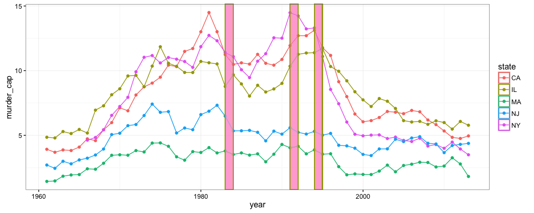
Just for visual effect I added some bars to demarcate important “Broken Windows” time periods: 1982-83 period, 1990-1991 period, and 1993-1994 period. 1982 was when the Kelling and Wilson article first appeared, 1990 the reign of Bratton over the NY Transit Authority, and 1993 the promotion of Bratton to NYPD Police Chief.

Some Future Stuff:

• The California crime data I got has violent crime and misdemeanors at the county level. I would like to work with this a little if I can figure out how to get number of police employed at the sub-state level.
• The data I pulled from BLS has police employment from 2005 to 2015. This won’t help us analyze data over the key “broken windows” time-frame (1990s) but I might use it to estimate a more general relationship between misdemeanor arrests and violent crime.