so I had some fun messing around with a new R package for doing AB Testing in a Bayesian framework. Here’s my report:

AB Testing

AB testing appears to me to be yet another way that people have tried to rebrand basic statistics. As far as I can tell ‘AB Testing’ just means asking whether A is better than B.

The nub of the problem is this:

• we have a current state of affairs (a red pill, 14 point font on the ‘click here’ button for a website, free school lunch) - the ‘A’ case
• we have an alternative treatment (a blue pill, 12 point font on the ‘click here’ button, etc)
• we want to design a controlled experiment to determine whether B is better than A

To fix ideas, the canonical problem we will consider here is this:

• we have a webpage with a ‘become a member’ button and we think we have some idea what the current success rate (the proportion of visitors who become members) is.
• we are considering a new page design and want to know if the new design will increase the success rate

The Frequentist Way

I’m gonna be pretty hand-wavey here because there are literally a thousand places you can go for primers on experimental design in the frequentist context. The basics are this:

Suppose we think the current success rate is 30%. We have a claim (from our product team) that the new page design will increase the success rate to 40%. In the frequentist universe we would:

• decide on a confidence level for our test (say $\alpha$ = 95%)
• decide on a power level (the probability of correctly detecting an effect size of 30%) for our test (say 80%)
• use the standard power calculators to determine how many study subjects in each group we need in order to be 95% confident the observed success rate for group B is 30% higher than the observed success rate for group A.

Some Bayesian Basics

The backbone of the frequentist methodology is rejecting the null hypothesis of 0 effect. I don’t want to get into a big thing about frequentists vs. Bayesian but, for the purposes of this post I will point out that many people find the interpretability of the frequentist approach unappealing.

The Bayesian approach proceeds by treating the underlying parameter value (the success rate) as a random variable with a distribution that can be inferred from the data…This contrasts with the frequentist approach of assuming the underlying population parameter value is fixed and all the uncertainty comes from sampling error.

In our example of Bayesian AB testing the quantity of most intense interest is the posterior distribuiton of the success rate.

Bayes Rule says:

is the prior probability of observing the parameter $\theta$ given the data, $X$.

is the likelihood of observing the data sample $X$ given the parameter $\theta$.

\(P(X)\) is the marginal probability of observing the data sample $X$.

This can be leveraged for AB testing in the following way. Suppose we belive the current success rate is 0.3. We want to test whether some webpage improvements will get us a success rate of 0.4.

In the Bayesian sense what we would like to do is show a bunch of people the original page and estimate the posterior distribution of the success rate. Then show a bunch of people the new webpage and estimate the posterior distribution of that success rate. Comparing the posterior distributions of two success rates will tell us whether we belive the success rate for the new page is better than the success rate for the old page.

The mechanics of Bayesian Stats are a little intimidating but the basic idea for AB testing can be distilled like so:

Given the current success rate of 0.3 and a data sample of a few hundred people who were shown the first page, the prior distribution of success rate is:

Let’s start with the likelihood:

Each individual either signs up or doesn’t so the likelihood of the data is a Bernoulli distribution with success rate $\theta$:

The prior is a little more complicated but let’s gloss over the complexity for now and just accept that we want a conjugate prior for the binomial distribution and sources tell us that the conjugate distribution for the binomial is the Beta distribution. So we will set our prior on $\theta$ to be,

where $B(a,b)$ is the Beta function.

Resources

There are lots of pretty informative posts on the interwebs about Bayesian AB Testing. I recommend the following:

this one has some fun quotes about Bayesian and Frequentist Statistics in an AB Testing Context.

Frank Portman is the author of an R Package to do Bayesian AB Testing.

This one is a bit long and round-about but does have some nice code chunk.

A quick guide to Thomson Sampling

Evan Miller has a pretty nice, compact post with most of the math you could ever want.

Some Bayesian Illustrations

For our numerical example we stated that we belive $\theta$ to be around 0.3. Let’s look at a couple beta distributions:

hist(rbeta(100,5,5))
hist(rbeta(100,50,50))
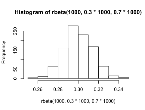
hist(rbeta(1000,0.3*1000,0.7*1000))

The variance of the beta distribution is controlled by the size of the shape parameters a and b. The parameters a and b can be thought of as the number of successes and failures in a + b trials.

Since we used a conjugate prior there is an analytical way to express the posterior distribution of $\theta$:

which is,

this post shows that this expression for the posterior is equivalent to a beta distribution with parameters $a’$ and $b’$ where

and

Let’s go ahead and step through this process from start-to-finish:

Step 1: simulate some data

Let’s start by simulating some data

X <- rbinom(100,1,0.3)
X
  [1] 0 0 0 1 1 0 0 0 0 1 0 0 1 0 0 1 0 0 1 1 0 0 0 0 1 1 0 1 1 0 0 0 0 1 0 0 1 0 0 0 0 0 0 0 1 0 0 0
 [49] 0 0 0 1 0 1 0 0 1 0 0 0 0 0 1 0 0 0 1 0 1 0 0 0 0 0 1 0 0 0 0 1 0 1 1 1 0 0 1 1 0 0 0 0 0 0 0 0
 [97] 0 0 1 0
 
sum(X)
> 28

Step 2: propose a prior

Suppose we belive the success rate is around 30% but we want a prior that is not too restrictive:

library(bayesAB)
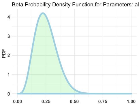
plotBeta(5,15)

Let’s see if we can find a prior that’s not too restrictive but centered more around 0.3

plotBeta(30,60)

Step 3: estimate the posterior

We showed above that with a beta prior and binomial likelihood we get a posterior distribution for this particular problem of:

with

and

For our case this leads to:

a <- 30 + sum(X)
b <- 60 + 100 - sum(X)

a
[1] 52

b
[1] 138

Step 4: plot the posterior

# 1,000 samples from the posterior distribution
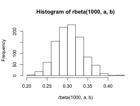
hist(rbeta(1000,a,b))

E_theta = a/(a+b)
var_theta = (a*b)/(((a+b)^2)*(a+b+1))

E_theta
var_theta

[1] 0.3052632
[1] 0.001110354

Let’s take a moment to appreciate what happened here. The initial prior on the success rate was that it would be distributed Beta(30,60) which maps to 30 success in 90 trials…an expected success rate of 0.333. From the data we observed 28 successes in 100 trials. The parameters of our distribuiton for the success rate were adjusted down to match the data and our estimated posterior distribution around the success rate has an expected value fo 0.3.

Step 5: Sensativity to priors

First, let’s wrap Steps 1 - 4 up into a function that we can call iteratively:

bayes.mams <- function(X, a.prior,b.prior){

  
  a.prime <-   a.prior + sum(X)
  b.prime <- b.prior + length(X) - sum(X)

  E_theta = a.prime/(a.prime+b.prime)
  var_theta = (a.prime*b.prime)/(((a.prime+b.prime)^2)*(a.prime+b.prime+1))
  
  return(list(E_theta,var_theta,rbeta(1000,a.prime,b.prime)))
  
}

Now let’s use this function to compare the data to the bayesian predicted posterior under a different choices of for the prior:

bayes <- bayes.mams(X=X,a.prior=1,b.prior=2)

# Success rate in the underlying data:
sum(X)/length(X)
[1] 0.28

# Expected value of the prior distribution
1/(1+2)

[1] 0.3333333

# Expected value of the posterior distribution:
bayes[[1]]

[1] 0.2815534

#plot the prior and posterior for a really diffuse prior
prior <- rbeta(1000,1,2)
post <- bayes.mams(X=X,a.prior=1,b.prior=2)[[3]]
plot.df <- data.frame(rbind(data.frame(x=prior,label='prior'),data.frame(x=post,label='posterior')))
ggplot(plot.df,aes(x=x,color=label)) + geom_density() + theme_bw()

Now do the whole thing again but make the prior a little more informative:

# Success rate in the underlying data:
sum(X)/length(x)
[1] 0.28

# Expected value of the posterior distribution:
post.tmp <- bayes.mams(X=X,a.prior=300,b.prior=600)
post.tmp[[1]]
[1] 0.328

#plot the prior and posterior for a = 300, b=600
prior <- rbeta(1000,300,600)
plot.df <- data.frame(rbind(data.frame(x=prior,label='prior'),data.frame(x=post.tmp[[3]],label='posterior')))
ggplot(plot.df,aes(x=x,color=label)) + geom_density() + theme_bw()

Summary

This seems to jive with my limited understanding of the Bayesian Machinery. Originally, we started with a prior of

This prior produces an expected success rate of 0.33. Our data sample produced a success rate of 0.28. When the prior was informed by the data, the posterior expected success rate fell to 0.3.

Next we tried a really flat prior,

which basically said, “eh, the success rate could be anything.” When we combined this really diffuse prior with the data, the data sample dominated the calculation of the posterior and we got a posterior expected value for the success rate that was pretty much exactly what was observed in the data sample.

Finally, we used a prior with even lower variance than either of the previous iterations. In this case, the prior expected success rate of 0.33 was moved only a tiny bit by the data sample - posterior expected success rate was only 0.32 when we observed 28 successes in 100 trial…because the prior was relatively restrictive.

Extension to Explicit AB Testing

To make the final jump from our last section to a traditional AB testing framework we just need to implement the steps above a few more times:

Suppose we believe that page A has a success rate of 0.3 and an improvement (page B) will offer a success rate of 0.4. We are going to test this on 1,000 visitors.

X <- rbinom(1000,1,0.3)
sum(X)/length(X)
[1] 0.29

Y <- rbinom(1000,1,0.4)
sum(Y)/length(Y)
[1] 0.41

b1 <-bayes.mams(X=X,a.prior=1,b.prior=2)
b2 <-bayes.mams(X=Y,a.prior=1,b.prior=2) 

b1[[1]]
[1] 0.2991

b2[[1]]
[1] 0.41

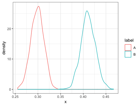
plot.df <- rbind(data.frame(x=b1[[3]],label='A'),data.frame(x=b2[[3]],label='B'))
ggplot(plot.df,aes(x=x,color=label)) + geom_density() + theme_bw()

How many sample in B are under the A curve?

sum(unlist(b2[[3]]) < max(unlist(b1[[3]])))/length(unlist(b2[[3]]))
[1] 0.0

We might interpret this as a 0% chance that the success rate for B is less than the success rate for A.

Quick Look at the bayesAB package

Now let’s see if the bayesAB package in R gives us something similar:

ab1 <- bayesTest(X, Y,
                 priors = c('alpha' = 1, 'beta' = 2),
                 n_samples = 1e5, distribution = 'bernoulli')

print(ab1)

--------------------------------------------
Distribution used: bernoulli 
--------------------------------------------
Using data with the following properties: 
            A     B
Min.    0.000 0.000
1st Qu. 0.000 0.000
Median  0.000 0.000
Mean    0.299 0.411
3rd Qu. 1.000 1.000
Max.    1.000 1.000
--------------------------------------------
Conjugate Prior Distribution: Beta 
Conjugate Prior Parameters: 
$alpha
[1] 1

$beta
[1] 2

--------------------------------------------
Calculated posteriors for the following parameters: 
Probability 
--------------------------------------------
Monte Carlo samples generated per posterior: 
[1] 1e+05

summary(ab1)

Quantiles of posteriors for A and B:

$Probability
$Probability$A
       0%       25%       50%       75%      100% 
0.2334814 0.2893877 0.2990061 0.3088185 0.3655146 

$Probability$B
       0%       25%       50%       75%      100% 
0.3488257 0.4001973 0.4105980 0.4211724 0.4887370 


--------------------------------------------

P(A > B) by (0)%: 

$Probability
[1] 0

--------------------------------------------

Credible Interval on (A - B) / B for interval length(s) (0.9) : 

$Probability
        5%        95% 
-0.3418837 -0.1946334 

--------------------------------------------

I’m sure the bayesAB package does a lot more cool stuff related to Bayesian AB Testing and maybe I’ll take a deeper look a little later. For now, it’s enough for me to know that summary results appear to be somewhat consistent with my rudimentary understanding of how to do ‘by hand.’