Social vulnerability indicators with r
Here is something I’ve been doing at work that I’m kinda proud of. It’s a fully reproducible spatial visualization of social vulnerability indicators by Census Tract for the West Coast. The entire project is available for download on my GitHub svi-tools repository here.
A pretty thorough walk-through exists here.
Background
Social Vulnerability refers to the resilience of communities when confronted by external stresses on human health, stresses such as natural or human-caused disasters, or disease outbreaks.
The Center for Disease Control, Environmental Protection Agency, Federal Emergency Management Agency, NOAA, and a ton of other state and federal government agencies use social vulnerability indicators for a variety of purposes…among them:
- The CDC and various state departments of health use social vulnerability indicators to scree for communities that may be of particularly high risk of disruption from disease outbreaks or other adverse public health events.
- The EPA uses social vulnerability indicators to construct their Environmental Justice Screener. Their Environmental Justice Screener is meant to identify and protect vulnerable communities from environmental hazards like water quality degredation.
- NOAA uses social vulnerability to identify communities that might be particularly adversely affected by commercial fisheries management policies.
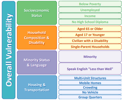
Social Vulnerability Indexes are generally constructed using data related to the following themes and metrics:
Problem
problem 1
The first problem or challenge that one normally encounters when trying to replicate or construct a Social Vulnerability Index is that the shear amount of data required is onerous in itself. There are 16 key metrics that feed into most Social Vulnerability Indicies. However, many of these metrics are aggregations of 10-20 primary data series.
For example, the indicator ‘No High School Diploma’ is generally constructed from The Census Bureau’s American Communities Survey table B15001. Most applications that I have encountered actually use for this metric, “Percent of the population 25 and over with some high school education but no diploma.” In order to contruct the metric “percent of population 25 and over with some high school education but no diploma”, one needs the individual data series:
- B15001_013E, males age 25-34 with some high school but no diploma
- B15001_021E, males age 35-44 with some high school but no diploma
- etc, etc,
- B15001_078E, females age 65 and up with some high school but no diploma
a total of 8 individual data series.
problem 2
The 2nd problem one generally encounters in the construction of a Social Vulnerability Index is that getting the necessary data series from the Census Bureau’s Data Web Mart, The American Fact Finder can be quite clunky. To get the data series mentioned above to calculate the metric, “Percent of the population 25 and over with some high school but no diploma” I follow these steps:
- select “Guided Search” from the landing page
- select “information about people”, then “educational attainment” from the Topics page
- select geography type: Census Tract, state: CA, county: all counties from the Geography page
- select “No, I’m not looking for race or ethic data” from the Race/Ethnic Groups page
- select table B15001 from the results page
What I get is a table with the educational attainment of 5 age groups broken down by gender. If I also select “Modify Table” –> “transpose” then I get a sensible looking table with Census Tracts along the rows and educational attainment estimates in the columns. Then I can export the results to a .csv file.
All-in it took me somewhere in the neighborhood of 5-8 minutes to get these data using the American Fact Finder…not terrible for one or two data series, but really annoying if you want like 20 or 30 data series.
problem 3
The biggest problem I have with getting all 50-odd primary data series necessary to contruct a Social Vulnerability Index using the American Fact Finder is that there are so many steps to follow that it’s REALLY hard to completely document all the steps in a way that makes your particular index reproducable.
Solution
I’ve written a library of R functions to automate all the data pulls necessary to construct the 16 social vulnerability indicators above. I’ve also written wrapper functions which sequentially call all of the data functions for any year, state, county, census tract, and/or census designated place.
This wasn’t particularly intellectually taxing but I think it represents a pretty solid contribution to social science research as it:
- makes the compilation of community social vulnerability indicies completely (and easily) reproducable.
- allows these indicators to be easily constructed for any geography (state, county, census tract, etc) and any year.
To illustrate the extent to which I’ve simplified the acquisition of social vulnerability indicators data from the Census Bureau, here is the minimum required to get a complete social vulnerability indicators data set for all Census Tracts in California using the American Communities Survey 5-year estimates for 2015.
Assuming you’ve pulled the file SVI_censustract_functions.R from my GitHub repo and assuming you have a key for Census Bureau’s API:
source('R/SVI_censustract_functions.R')
key <- ''

#call the svi census tract function to build the data
svi.df <- svi_data_censustract.fn(yr=2015,key=key)

#save the results locally so you don't have to recompile every time
saveRDS(svi.df,file='svi_censustract_2015.RDA')
I’m not gonna lie to you, the initial data compilation isn’t quick. But if you’re willing to wait 20 minutes you get a fully formed SVI data set at the Census Tract level:
head(svi.df)
                                          name total_households state county  tract total_pop
1 Census Tract 4001, Alameda County, California             1286    06    001 400100      2952
2 Census Tract 4002, Alameda County, California              832    06    001 400200      1984
3 Census Tract 4003, Alameda County, California             2489    06    001 400300      5377
4 Census Tract 4004, Alameda County, California             1801    06    001 400400      4105
5 Census Tract 4005, Alameda County, California             1624    06    001 400500      3651
6 Census Tract 4006, Alameda County, California              701    06    001 400600      1665
     pov.pct unemp.rate pop25 edu25 pct_no_diploma    pci no_health_insurance pop_under_65
1 0.03489160 0.05656425  2420    40     0.01652893 104852                  95         2273
2 0.05796371 0.02575897  1611    24     0.01489758  76930                 104         1543
3 0.08097928 0.09389810  4338   216     0.04979253  62892                 213         4635
4 0.07440839 0.03503309  3346   204     0.06096832  53779                 144         3585
5 0.12654746 0.06431005  2913    93     0.03192585  38442                 439         3297
6 0.06602059 0.14502370  1276   100     0.07836991  37911                 213         1459
  pct_no_healthins pop_under_18 pop_over_65 disable_pct single_mom_pct pct.nonwhite pct_limited_eng
1       0.04179498          440         579  0.05426028     0.03810264    0.2801491      0.03810264
2       0.06740117          318         356  0.02234994     0.02524038    0.1980847      0.00000000
3       0.04595469          899         582  0.04734485     0.06588992    0.3384787      0.08879068
4       0.04016736          654         428  0.09493671     0.05330372    0.2874543      0.02332038
5       0.13315135          443         269  0.06891408     0.09913793    0.3815393      0.02278325
6       0.14599040          204         171  0.06534653     0.13266762    0.6180180      0.01283880
  housing_gt_10_pct mobile_pct pct_crowded pct_no_vehicle   pct_group
1        0.00000000          0 0.006550218     0.01310044 0.000000000
2        0.09479769          0 0.000000000     0.05664740 0.044354839
3        0.25242718          0 0.000000000     0.14058252 0.006323229
4        0.10903260          0 0.008017103     0.06841261 0.014372716
5        0.18063754          0 0.023612751     0.13990555 0.000000000
6        0.02432432          0 0.028378378     0.21216216 0.005405405
technical detail
As a prerequisite you will want to check out my previous post on automating Census Bureau data acquisition with R. This post contains the basics of setting up an API key and a little jump-start into pulling Census Bureau data with R.
Setting up the data function library was mostly grunt-work, not super glamorous. Basically, I just identified all the individual data series that one would need in order to compile the 16 aforementioned indicators and created a function to pull each one for a given year and state. An example of one such function to get portion of the population with income below the poverty line in last 12 months is,
#first create a function to generate the appropriate API call
library(RJSONIO)
library(rgdal)
library(ggplot2)
library(ggmap)
library(scales)
library(maptools)
library(rgeos)
library(dplyr)
library(data.table)


api_call.fn <- function(year,state,series,key){


if(year %in% c(2009,2010)){
  call <- paste('https://api.census.gov/data/',year,'/acs5?key=',key,'&get=',series,',NAME&for=tract:*&in=state:',state,
                 sep="")
}else if(year %in% c(2011,2012,2013,2014)){
  call <- paste('https://api.census.gov/data/',year,'/acs5?get=NAME,',series,'&for=tract:*&in=state:',state,'&key=',
                 key,sep="")
}else{
  call <- paste('https://api.census.gov/data/',year,'/acs/acs5?get=NAME,',series,'&for=tract:*&in=state:',state,'&key=',
                 key,sep="")

}

return(call)
}


# A function to get percent of households below the poverty line from the ACS 5 year
# estimates for a particular year

#------------------------------------------------------------------------------
# population for which poverty status is determined B17001_001E
# population with income below the poverty line in the last 12 months B17001_002E

below_poverty.fn <- function(state,year,key){

series1 <- 'B17001_001E'
series2 <- 'B17001_002E'

call1 <- api_call.fn(year=year,state=state,key=key,series=series1)
call2 <- api_call.fn(year=year,state=state,key=key,series=series2)


# population for whom poverty status is determined
pov.pop <- fromJSON(call1)
pov.pop <- data.frame(rbindlist(lapply(pov.pop,function(x){
  x<-unlist(x)
  return(data.frame(name=x[1],pov.pop=x[2],state=x[3],county=x[4],tract=x[5]))
})
)) %>% filter(row_number() > 1)


# income in the past 12 months below poverty level
pov <- fromJSON(call2)
pov <- data.frame(rbindlist(lapply(pov,function(x){
  x<-unlist(x)
  return(data.frame(name=x[1],pov=x[2],state=x[3],county=x[4],tract=x[5]))
})
)) %>% filter(row_number() >1)

pov <- tbl_df(pov) %>% inner_join(pov.pop,by=c('name','state','county','tract')) %>%
  mutate(pov.pct = as.numeric(as.character(pov))/as.numeric(as.character(pov.pop)))

return(pov)
}
A slightly more intense example involves the metric we talked about previously, “population age 25 and over with some high school education but no diploma”:
#--------------------------------------------------------------------------------
# education - population 25 and over with less than a high school degree

edu.fn<-function(year,state,key){

  series.df <- data.frame(series=c(
    'B15001_013E','B15001_021E',
    'B15001_029E','B15001_037E',
    'B15001_054E','B15001_062E',
    'B15001_070E','B15001_078E'),
    labels=c('m_25_34_nodiploma','m_35_44_nodiploma',
             'm_45_64_nodiploma','m_65_plus_nodiploma',
             'f_25_34_nodiploma','f_35_44_nodiploma',
             'f_45_64_nodiploma','f_65_plus_nodiploma'))

    counts.df <- data.frame(series=c('B15001_011E','B15001_019E','B15001_027E','B15001_035E',
                                   'B15001_052E','B15001_060E','B15001_068E','B15001_076E'),
                          labels=c('m_25_34','m_35_44','m_45_64','m_65_plus',
                                   'f_25_34','f_35_44','f_45_64','f_65_plus'))
tmp.df <- list()
for(i in 1:nrow(series.df)){
  call1 <- api_call.fn(year=year,state=state,key=key,series=series.df$series[i])
  call2 <- api_call.fn(year=year,state=state,key=key,series=counts.df$series[i])

  total.age <- fromJSON(call2)
  total.age <- data.frame(rbindlist(lapply(total.age,function(x){
    x<-unlist(x)
    return(data.frame(name=x[1],pop.age=x[2],state=x[3],county=x[4],tract=x[5]))
  })
  )) %>% filter(row_number() > 1)

  edu.age <- fromJSON(call1)
  edu.age <- data.frame(rbindlist(lapply(edu.age,function(x){
    x<-unlist(x)
    return(data.frame(name=x[1],edu.age=x[2],state=x[3],county=x[4],tract=x[5]))
  })
  )) %>% filter(row_number() > 1)

  z <- edu.age %>% inner_join(total.age,by=c('name','state','county','tract')) %>%
         mutate(age.range=as.character(counts.df$labels[i]))
tmp.df[[i]] <- z
}

edu<- data.frame(rbindlist(tmp.df)) %>%
      group_by(name,state,county,tract) %>%
      summarise(no_diploma=sum(as.numeric(as.character(edu.age)),na.rm=T)
                ,pop=sum(as.numeric(as.character(pop.age)),na.rm=T)) %>%
     mutate(pct_no_diploma=no_diploma/pop)

return(edu)
}
#--------------------------------------------------------------------------------------------
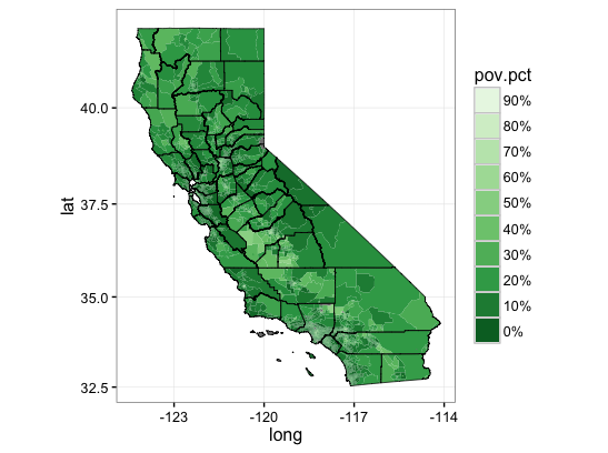
Cool Extension
In this post I demo’d some mapping with Census Bureau shapefiles. In my new social vulnerability tools GitHub repository I’ve included all the census tract boundary and county boundary shapefiles for California. If you grab these you should be able to reproduce the following visualizations of Census Bureau social vulnerability data rather easily:
rm(list=ls())

library(rgdal)
library(ggplot2)
library(ggmap)
library(scales)
library(maptools)
library(rgeos)
library(dplyr)

############################################################################################################
############################################################################################################
############################################################################################################
############################################################################################################
############################################################################################################
############################################################################################################
############################################################################################################
############################################################################################################


############################################################################################################
############################################################################################################
############################################################################################################
############################################################################################################
############################################################################################################
############################################################################################################
############################################################################################################
############################################################################################################
# A regional mapping exercise

svi.df <- readRDS('data/svi_censustract_2015.RDA')

tract <- readOGR(dsn = "shapefiles/gz_2010_06_140_00_500k",
                 layer = "gz_2010_06_140_00_500k")
tract <- fortify(tract, region="GEO_ID")

# the GEO ID for a census tract is state + county + tract...
# state must have the trailing 0
# county must be 3 digit
ca.poverty <- tbl_df(svi.df) %>%
              select(name,state,county,tract,pov.pct) %>%
              filter(state=='06') %>%
              mutate(id=paste('1400000US',state,county,tract,sep=""))


plotData <- left_join(tract,ca.poverty)

county <- readOGR(dsn = "shapefiles/gz_2010_06_060_00_500k",
                  layer = "gz_2010_06_060_00_500k")
county <- fortify(county, region="COUNTY")

#now I'm going to use the scales() package to bin the data a little
# so the contrasts in coverage rates are a little more visible
ggplot() +
  geom_polygon(data = plotData, aes(x = long, y = lat, group = group,
                                    fill = pov.pct)) +
  geom_polygon(data = county, aes(x = long, y = lat, group = group),
               fill = NA, color = "black", size = 0.25) +
  coord_map() +
  scale_fill_distiller(palette = "Greens", labels = percent,
                       breaks = pretty_breaks(n = 10)) +
  guides(fill = guide_legend(reverse = TRUE)) + theme_bw()
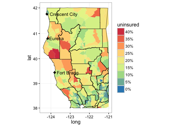
And here is one where I zoomed in on California’s North Coast area and displayed percent of population without health insurance.
ca.ins <- tbl_df(svi.df) %>%
  select(name,state,county,tract,pct_no_healthins) %>%
  filter(state=='06') %>%
  mutate(id=paste('1400000US',state,county,tract,sep="")) %>%
  mutate(uninsured=pct_no_healthins)


plotData <- left_join(tract,ca.ins)


#now try just a zoom on some North Coast areas
# a few reference points
point.df <- data.frame(name=c('Crescent City','Fort Bragg','Eureka'),
                       lat=c(41.7558,39.4457,40.8021),
                       long=c(-124.2026,-123.8053,-124.1637))

ggplot() +
  geom_polygon(data = subset(plotData,lat>=38 & long<=-121), aes(x = long, y = lat, group = group,
                                                                 fill = uninsured)) +
  geom_polygon(data = subset(county,lat>=38 & long<=-121), aes(x = long, y = lat, group = group),
               fill = NA, color = "black", size = 0.25) +
  geom_point(data=point.df,aes(x=long,y=lat),shape=18,size=3) +
  geom_text(data=point.df,
             aes(x=long,y=lat,label=name),hjust=-0.1) +
  coord_map() +
  scale_fill_distiller(palette = "Spectral", labels = percent,
                       breaks = pretty_breaks(n = 10)) +
  guides(fill = guide_legend(reverse = TRUE)) + theme_bw()