Automating census data pulls with r
I had a pretty cool little quantitative micro-targeting of policy issues model I wanted to show you guys today. But I had to get this Census Bureau API-R relationship smoothed out for a work thing and I’m kinda thinking it will have more universal appeal. So I’m posting it first.
Here is the gist: The Census Bureau collects lots of really cool data: demographic, socio-economic, social structure type stuff:
- educational attainment by state, congressional district, city, census tract, ext
- percent of population speaking a language other than English at home…by state, census tract, school district, whatever
- number of homeowners versus renters by various geographies
I know everybody is all beside themselves about using Twitter/Facebook/whatever for some micro-analysis. But we shouldn’t forget that for a lot of applications (political issue tracking, environmental justice, economic development) we can get a lot of milage out of the stuff the Census Bureau already collects.
The rub is that the Census Bureau’s data organization is kinda poor and their web GUIs for data retrieval are really confusing and hard to use.
Most of the stuff in this post will rely on API calls rather than static data files…but there are a few .csv files you may want and the full annotated R code is also available here:
Aaron’s R Spatial GitHub Repo.
Pulling Census Data in R
Have you ever wanted to know how many people in your city speak Taglog at home? Or how many black people live in Vermont? Or what percent of the people in Jackson, Mississippi have a college degree? Then the American Fact Finder web GUI is for you.
But if you’ve ever wondered how the age structure of Franklin County, TN has changed over the last 7 years (perhaps as job opportunities in rural areas continue to decline and young people increasingly migrate to urban areas) AND you’d like to compare that change to changes in other rural geographies in the U.S. AND you’d like your analysis to be reproducible AND possibly applicable to other similar research questions…then you owe it to yourself to get friendly with the Census Bureau’s API.
Here’s a great resources that I borrowed from pretty heavily
Prerequisites
There are two crucial prerequisites for this section:
-
An API key from the Census Bureau…get one here
-
The R package RJSONIO.
A quick word on item 2: there is an R package called acs or something like that which is designed to work with data from the Census Bureau’s American Communities Survey. Try it out if you want. I monkeyed with it but found it was overkill. The fromJSON() function in the RJSONIO library is pretty much all I need…or want for that matter
An Example
The sample API call on the Census Bureau’s Developers page to get population by state from the 1 year estimates of the 2015 American Communities Survey is:
api.census.gov/data/2015/acs1?get=NAME,B01001_001E&for=state:*&key=…
In the code below I pass this API call to the Census Bureau, use the fromJSON() function to collect the JSON results in an R list, and clean up the list
library(RJSONIO)
key <- mykey
resURL <- paste('http://api.census.gov/data/2015/acs1?get=NAME,B01001_001E&for=state:*&key=',
+                 key,sep="")
ljson<-fromJSON(resURL)
head(ljson)
[[1]]
[1] "NAME"        "B01001_001E" "state"

[[2]]
[1] "Alabama" "4858979" "01"

[[3]]
[1] "Alaska" "738432" "02"

[[4]]
[1] "Arizona" "6828065" "04"

[[5]]
[1] "Arkansas" "2978204"  "05"

[[6]]
[1] "California" "39144818"   "06"
I can drop this into a dataframe pretty easily with:
ljson<-ljson[2:length(ljson)]
pop <- data.frame(statename=unlist(lapply(ljson,function(x){x[1]})),
                  totalpop=unlist(lapply(ljson,function(x){x[2]})),
                  state=unlist(lapply(ljson,function(x){x[3]})))
head(pop)
   statename totalpop state
1    Alabama  4858979    01
2     Alaska   738432    02
3    Arizona  6828065    04
4   Arkansas  2978204    05
5 California 39144818    06
6   Colorado  5456574    08
Another Example
I like examples. Especially when you are coding, I think it’s hyper-useful to have a stock of examples. It ups the probability that, for whatever specific thing you want to do, you’ll just have to alter a couple lines of existing code.
Here’s what’s going on in this example:
- I used the API call to pull total Hispanic population by congressional district for the U.S.
- used a separate API call to pull total population by congressional district for the U.S.
- combined those 2 to create the % Hispanic population in each congressional district
- merged that with results of the 2016 Congressional Elections
#set up the API call for Hispanic Population by Congressional District
resURL <- paste("http://api.census.gov/data/2015/acs1?get=NAME,B01001I_001E&for=congressional+district:*&key=",
                key,sep="")
latinos <- fromJSON(resURL)
latinos <- latinos[2:length(latinos)]

#Set up the API call for total population
resURL <- paste("http://api.census.gov/data/2015/acs1?get=NAME,B01001_001E&for=congressional+district:*&key=",
                key,sep="")
pop <- fromJSON(resURL)
pop <- pop[2:length(pop)]
pop.L <- data.frame(name=unlist(lapply(pop,function(x){unlist(x)[1]})),
                    pop=unlist(lapply(pop,function(x){unlist(x)[2]})),
                    state=unlist(lapply(pop,function(x){unlist(x)[3]})),
                    cd=unlist(lapply(pop,function(x){unlist(x)[4]})))

latinos <- data.frame(name=unlist(lapply(latinos,function(x){unlist(x)[1]})),
                      latino.pop=unlist(lapply(latinos,function(x){unlist(x)[2]})))

pop.L <- pop.L %>% inner_join(latinos,by=c('name')) %>%
            mutate(pct_latino=as.numeric(as.character(latino.pop))/
                     as.numeric(as.character(pop)))

#get the 2016 Congressional Election results
house_election_2016 <- read.csv('data/congressionalelections2016.csv')
#get the numeric codes for each state
state.codes <- read.csv('data/state_fips_codes.csv')
names(state.codes) <- c('statename','state.num','state')

votes <- house_election_2016 %>%
          inner_join(state.codes,by=c('state'))

#fix pop.L congressional districts
pop.L$cd <- as.numeric(as.character(pop.L$cd))
pop.L$state <- as.numeric(as.character(pop.L$state))

votes <- votes %>% select(state.num,cd,winning_party)
names(votes) <- c('state','cd','party')

votes <- votes %>% inner_join(pop.L,by=c('state','cd'))

#order it by latino population and see if there are any notable 'R's
votes %>% arrange(-pct_latino)

   state cd party                                                     name    pop latino.pop pct_latino
1      6 21     R   Congressional District 21 (114th Congress), California 716371     535377 0.74734600
2     48 23     R        Congressional District 23 (114th Congress), Texas 747732     521424 0.69734076
3     12 26     R      Congressional District 26 (114th Congress), Florida 776959     541186 0.69654383
4      6 10     R   Congressional District 10 (114th Congress), California 739784     316229 0.42746126
5      6 25     R   Congressional District 25 (114th Congress), California 720316     268191 0.37232409
6      6 24     D   Congressional District 24 (114th Congress), California 736757     264994 0.35967626
7     32  4     D        Congressional District 4 (114th Congress), Nevada 722406     201492 0.27891795
8      6 49     R   Congressional District 49 (114th Congress), California 735828     189640 0.25772327
9      8  3     R      Congressional District 3 (114th Congress), Colorado 737812     181423 0.24589326
10     4  1     D       Congressional District 1 (114th Congress), Arizona 759663     173716 0.22867508
11    17 10     D     Congressional District 10 (114th Congress), Illinois 714251     160421 0.22460032
12    12  7     D       Congressional District 7 (114th Congress), Florida 738367     157720 0.21360651
13     8  6     R      Congressional District 6 (114th Congress), Colorado 796156     163880 0.20583906
14    32  3     D        Congressional District 3 (114th Congress), Nevada 758676     125431 0.16532881
15     6  7     D    Congressional District 7 (114th Congress), California 739069     117592 0.15910828
16     6 52     D   Congressional District 52 (114th Congress), California 755498     118641 0.15703682
17    12 18     R      Congressional District 18 (114th Congress), Florida 748028     111507 0.14906795
18    36  1     R      Congressional District 1 (114th Congress), New York 726589     107873 0.14846495
19    51 10     R     Congressional District 10 (114th Congress), Virginia 807670     105618 0.13076875
20    34  5     D    Congressional District 5 (114th Congress), New Jersey 743424      94463 0.12706477
21    20  3     R        Congressional District 3 (114th Congress), Kansas 755396      88598 0.11728683
22    31  2     R      Congressional District 2 (114th Congress), Nebraska 652870      71614 0.10969106
23    36  3     D      Congressional District 3 (114th Congress), New York 721764      74127 0.10270255
24    12 13     D      Congressional District 13 (114th Congress), Florida 716429      72211 0.10079296
25    36 19     R     Congressional District 19 (114th Congress), New York 705044      51710 0.07334294
26    19  3     R          Congressional District 3 (114th Congress), Iowa 812464      54484 0.06706020
27    27  2     R     Congressional District 2 (114th Congress), Minnesota 695029      40193 0.05782924
28    55  8     R     Congressional District 8 (114th Congress), Wisconsin 727491      36678 0.05041712
29    42  8     R  Congressional District 8 (114th Congress), Pennsylvania 707083      35083 0.04961652
30    26  8     R      Congressional District 8 (114th Congress), Michigan 728781      35125 0.04819692
31    36 24     R     Congressional District 24 (114th Congress), New York 708959      31211 0.04402370
32    27  3     R     Congressional District 3 (114th Congress), Minnesota 700121      30328 0.04331823
33    26  7     R      Congressional District 7 (114th Congress), Michigan 697627      29680 0.04254422
34    19  1     R          Congressional District 1 (114th Congress), Iowa 771888      28650 0.03711678
35    36 23     R     Congressional District 23 (114th Congress), New York 708372      26115 0.03686622
36    36 22     R     Congressional District 22 (114th Congress), New York 711391      26099 0.03668728
37    33  1     D Congressional District 1 (114th Congress), New Hampshire 671640      24624 0.03666250
38    18  9     R       Congressional District 9 (114th Congress), Indiana 741982      24680 0.03326226
39    36 21     R     Congressional District 21 (114th Congress), New York 710842      23524 0.03309315
40    17 12     R     Congressional District 12 (114th Congress), Illinois 699369      23119 0.03305694
41    26  1     R      Congressional District 1 (114th Congress), Michigan 700136      13902 0.01985614
42    27  8     D     Congressional District 8 (114th Congress), Minnesota 663670      11133 0.01677490
43    23  2     R         Congressional District 2 (114th Congress), Maine 657319       8938 0.01359766
>
I didn’t really do this for any reason other than it sounded fun…but it does seem pretty interesting that the top congressional districts ranked by latino population are represented by Republicans…Although it deserves mention that I didn’t do any voting age population filters or anything like that here. It’s pretty off-the-cuff. But interesting nonetheless.
The Shitty Stuff
After toggling my way through the Census Bureau’s data GUI a few times to try and find basic shit like population, educational attainment, etc., I loved working with the API. However, the drawback to automating data retrieval with the API is that you have to know what series you are looking for. The Census Bureau does not make this easy.
Here is an example of where the API is still cool…but maybe not SUPER cool:
Suppose I want population by age and sex for each state in the U.S. and I start with the American Fact Finder. I can use either the ‘guided search’ or ‘advanced search’ to work my way through several filtering screens and arrive at an html table that will have a row/column (depending on how I decide to format the web query output) for each state and a row/column for each of like 100 variables (total population, total male population, males ages 5 and under, males ages 5-17, males ages 18-19,….total females, females ages 5 and under, etc., etc.). I can choose to download this table into a .csv format.
Alternatively, I can try to save myself several points and clicks and get the same data using the API. Here’s the rub: when I used the web tool I discovered that this particular table was Table B01001. THERE IS NO API CALL FOR TABLE B01001. There is an API call for:
- B01001_002E - total male population
- B01001_007E - total males ages 18 and 19
- B01001_026E - total female population
- B01001_040E - females age 50-54
Basically, using the API requires you to not only know the precise table you want but also the precise data series within that table.
Here is how I got 2012, 2014, and 2015 population by age and sex for each congressional district disregarding ages under 18 and over 55:
series.males <- c('001E','002E','007E','008E','009E','010E','011E','012E','013E','014E','015E','016E')
series.females <- c('026E','031E','032E','033E','034E','035E','036E','037E','038E','039E','040E')
series <- c(series.males,series.females)

series <- paste('B01001_',series,sep="")
series.names<- c('total pop','total male','m18_19','m20','m21','m22_24','m25_29','m30_34',
                 'm35_39','m40_44','m45_49','m50_54','total female','f18_19','f20','f21','f22_24',
                 'f25_29','f30_34',
                 'f35_39','f40_44','f45_49','f50_54')


pop.fn <- function(i,yr){
resURL <- paste('http://api.census.gov/data/',yr,
                '/acs1?get=NAME,',
                series[i],'&for=congressional+district:*&key=',key,sep="")
ljson <- fromJSON(resURL)
ljson <- ljson[2:length(ljson)]
tmp <- data.frame(unlist(lapply(ljson,function(x)x[1])),
                  unlist(lapply(ljson,function(x)x[2])),
                  unlist(lapply(ljson,function(x)x[3])),
                  unlist(lapply(ljson,function(x)x[4])),
                  series.names[i])
names(tmp) <- c('name','variable','state','congressional district','series_name')
return(tmp)
}

pop.df2015 <- data.frame(rbindlist(lapply(c(1:length(series)),pop.fn,yr=2015)))
pop.df2015$source <- 'ACS 2015 1 yr'
pop.df2014 <- data.frame(rbindlist(lapply(c(1:length(series)),pop.fn,yr=2014)))
pop.df2014$source <- 'ACS 2014 1 yr'
pop.df2012 <- data.frame(rbindlist(lapply(c(1:length(series)),pop.fn,yr=2012)))
pop.df2012$source <- 'ACS 2012 1 yr'
I don’t have much wisdom to offer on how to efficiently search for the precise series you are looking for (e.g. B01001_032E). I will tell you what I have found to be wildly inefficient: opening the variables list html table and doing a command+f search for some keyword. There are over 62,000 data series in the summary tables and another ~60,000 in the subject tables and my chrome browser hangs up for minutes trying to search the html table.
I haven’t totally flushed this out yet but I was able to use R’s XML package to read the variable list html table into R.
##################################################################
#Try to parse out the variables list so I can do some manner
# of informed search for searies I'm looking for:
library(XML)
theurl <- "http://api.census.gov/data/2015/acs1/variables.html"
tables <- readHTMLTable(theurl)

#################################################################
From here there is an object called Concept. This field has keywords that can help you narrow your search for the right series. At this point I’m not entirely sure how to access this object…but I do know that Concept has keywords like ‘Educational Attainment’ which can, at least in theory, help you locate the stuff you want.
A Mapping Example
Now, I want to combine some of the stuff I showed off in my last post. Specifically, I’m going to use the API to pull educational attainment for a chunk of western states at the geographic unit of congressional districts and crank out a map.
################################################################
################################################################
################################################################
# A quick mapping example

library(rgdal)
library(ggplot2)
library(ggmap)
library(scales)
library(maptools)
library(rgeos)
library(dplyr)

#use the function I wrote above to pull total population and population with a
# bachelors degree by congressional district from Census Bureau

edu.fn <- function(yr){
  resURL <- paste('http://api.census.gov/data/',yr,
                  '/acs1/subject?get=NAME,S1501_C01_006E&for=congressional+district:*&',
                  'key=f5a32f694a14b28acf7301f4972eaab8551eafda',sep="")
  ljson <- fromJSON(resURL)
  name <- unlist(lapply(ljson[2:length(ljson)],function(x)x[1]))
  pop25 <- unlist(lapply(ljson[2:length(ljson)],function(x)x[2]))
  state <- unlist(lapply(ljson[2:length(ljson)],function(x)x[3]))
  congressional_district <- unlist(lapply(ljson[2:length(ljson)],function(x)x[4]))
  df <- data.frame(name=name,pop25=value,state=state,congressional_district=congressional_district,
                   source=paste('ACS_1yr_',yr,sep=""))

  #add in the number of people 25 and over with a bachelor's degree
  resURL <- paste('http://api.census.gov/data/',yr,
                  '/acs1/subject?get=NAME,S1501_C01_012E&for=congressional+district:*&',
                  'key=f5a32f694a14b28acf7301f4972eaab8551eafda',sep="")
  ljson <- fromJSON(resURL)
  pop25_bachelors <- unlist(lapply(ljson[2:length(ljson)],function(x)x[2]))

  df$pop25_bachelors <- pop25_bachelors
  return(df)
}

#get educational attainment from the 2015 ACS
edu2015 <- edu.fn(yr=2015)

#read the shapefile with cartographic boundaries for congressional districts
#let's see if we can map some shit by congressional district
congress <- readOGR(dsn = "data/cb_2015_us_cd114_500k",
                    layer = "cb_2015_us_cd114_500k")
#pull out state, CD, and AFFGEOID so we can merge with the education stuff
df.tmp <- congress@data[,c('STATEFP','CD114FP','AFFGEOID')]
df.tmp$state_cd <- paste(df.tmp$STATEFP,df.tmp$CD114FP,sep="")

congress <- fortify(congress, region="AFFGEOID")

#keep edu from some western states (CA, AZ, NV, UT)
edu.tmp <- edu2015 %>% mutate(state_cd=paste(state,congressional_district,sep="")) %>%
            inner_join(df.tmp,by=c('state_cd')) %>%
            filter(state %in% c('06','04','49','32')) %>%
            rename(id=AFFGEOID) %>%
            mutate(pct_college=as.numeric(as.character(pop25_bachelors))/
                     as.numeric(as.character(pop25)))

plotData <- inner_join(congress,edu.tmp)

#trim the congress data frame
ids <- unique(edu.tmp$id)
congress <- congress %>% filter(congress$id %in% ids)

ggplot() +
  geom_polygon(data = plotData, aes(x = long, y = lat, group = group,
                                    fill = 1-pct_college)) +
  geom_polygon(data = congress, aes(x = long, y = lat, group = group),
               fill = NA, color = "black", size = 0.25) +
  coord_map() +
  scale_fill_distiller(palette = "YlOrRd", labels = percent,
                       breaks = pretty_breaks(n = 15)) +
  guides(fill = guide_legend(reverse = FALSE)) + theme_bw()
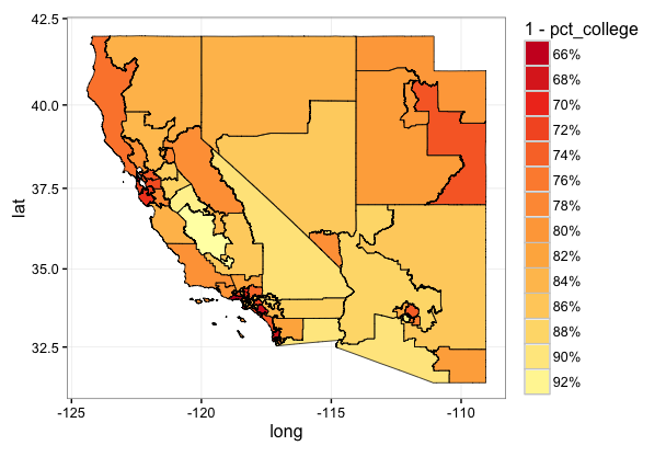
Ok, so the map is a little campy and maybe not super informative without some city-type context. It’s also probably worth noting that here I plotted 1 - percent of age 25 and over population wiht a Bachelor’s Degree. I wanted to display the education ‘hotspots’ in the darkest shades but didn’t want to spend all day monkeying with the palette brewer…so the darker reds are the congressional districts where relatively more of the population holds Bachelor’s Degrees.
I’m pretty sure there is some really cool quantitive policy I could do with this ability to quickly pull data Census data at the Congressional District level with the API and map it in R. Hopefully, I’ll be able to illustrate some of the analysis I have in mind in the next few blog posts.
I’ll try one more with a static google map basemap just to see what it looks like:
One last map…I promise
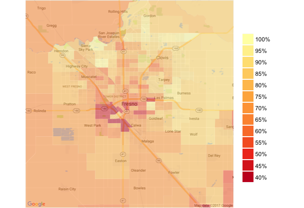
This one comes directly from Kevin Johnson’s blog post on clipping static Google maps to Census Bureau boundaries to create basemaps. Here I’m reverting back to the Census Tract boundaries and the percent of population with health insurance for California that I used in my last post. I’ll work on amending this to work with the Congressional District Boundaries later today.
Note that I’m using a pretty tight zoom around Fresno California. That’s because the larger the extent of the map, the less you will see of the features on the underlying basemap….and if the map is so big that you can’t see the word Fresno it doesn’t really make a ton of sense to add a context-rich basemap at all.
################################################################
################################################################
################################################################
#try it with a base map

#load the raster library
library(raster)

#go back to California Census Tract data because the map
tract <- readOGR(dsn = "data/gz_2010_06_140_00_500k",
                 layer = "gz_2010_06_140_00_500k")
#load back in the insurance data we pulled
ins <- read.csv("data/CA_insured_tract.csv")
ins$id <- as.character(ins$GEO.id)
ins$percent <- ins$Insured18_64/ins$Pop18_64

#get a basemap
map <- get_map("Fresno", zoom = 11, maptype = "roadmap")
p <- ggmap(map)
p

#establish a bounding box around our static google map
box <- as(extent(as.numeric(attr(map, 'bb'))[c(2,4,1,3)] +
                   c(.001,-.001,.001,-.001)), "SpatialPolygons")
proj4string(box) <- CRS(summary(tract)[[4]])
tractSub <- gIntersection(tract, box, byid = TRUE,
                          id = as.character(tract$GEO_ID))
tractSub <- fortify(tractSub, region = "GEO_ID")
plotData <- left_join(tractSub, ins, by = "id")

ggmap(map) +
  geom_polygon(data = plotData, aes(x = long, y = lat, group = group,
                                    fill = percent), colour = NA, alpha = 0.5) +
  scale_fill_distiller(palette = "YlOrRd", breaks = pretty_breaks(n = 10),
                       labels = percent) +
  labs(fill = "") +
  theme_nothing(legend = TRUE) +
  guides(fill = guide_legend(reverse = TRUE, override.aes =
                               list(alpha = 1)))