I found this post on the interwebs and thought it was pretty cool. I mean, I’m not enamored with the whole, “don’t worry about understanding what it’s doing, just run the code and get a feel for how to do it” vibe…as a practicing empiricist I’m pretty well aware of the fact that anyone can run the same R/Python/whatever code that I use to run a Neural Network, Support Vector Machine, Classification-and-Regression Tree, insert hip new ensemble method here. The thing that makes me worth anything at all - if I am indeed worth anything - isn’t that I know how to tell R to train a Neural Network, it’s that I know what the code is doing when I give it that command. I have a decent (a little better than most, a lot worse than a few) grasp of the technical detail and nuance (read: the math) of the popular machine learning and applied statistical algorithms used to do prediction.

Anyway, for those who are familiar with the techniques and models, I thought this Python tutorial was a really cool, condensed way to introduce the Python way to do things. Basically, it’s a couple lines of Python code that call machine learning functionalities in the scikit-learn module.

The Classifiers

• KNN - K nearest neighbor classifier
• CART - classification and regression tree
• NB - Gaussian Naive Bayes classifier
• LDA - Linear Discriminant Analysis
• LR - Logistic Regressin
• SVM - Support Vector Machines

I wrote a little bit about logistic regression and linear discriminant analysis last week. If I get some time later this week I’ll try to write some more in-depth shit about the other classifiers on this list…for now here’s the general idea of what these animals are:

KNN

K nearest neighbor classifiers are pretty much what they sound like: for any data set with outcomes in two classes $Y_{i} \in [0,1]$ and inputs $x=[x_{i1},x_{i2},…x_{in}]$ the KNN algorithm predicts that observation $j$ will belong to the same class as it’s K-nearest neighbors.

CART - Classification and Regression Trees

Hastie, Tibshirhani, and Friedman Chapter 9.2 contains the kernel of critical knowledge on tree based methods. This is really reductionist way to think about it but I like the example of housing prices because it has two interesting features:

1. we often suspect the relationships between inputs (bedrooms, bathrooms, location, locational amenities, etc) and outputs (home price) to be non-linear

2. we often suspect that the marginal effect of an input varies over the range of the input space.

Regression trees look for ways to partition the input space into subspaces where the input-output relationship is locally linear and stable.

The classic push/pull of overfitting versus and underfitting (accepting a model that does not account for important systematic sources of variation) is pretty simple to conceptualize in the case of a CART model. There is a surefire way to achieve near perfect fit with a CART model which is to make every data point it’s own node. This approach probably wouldn’t generalize well and would most likely produce plenty of prediction error. On the other hand, a tree with too few nodes is likely to fail to capture important structure in the data set and again will probably produce sizeable prediction errors.

Naive Bayes

I gave a little mini-course on Naive Bayes classifiers for sentiment analysis here. No need to rehash it here.

LDA and SVM

For classification problems where the goal is the predict what group an observation belongs to based on a set of observed characteristics (covariates, features, inputs, etc), Linear Discriminant Analysis (LDA) assumes that covariates are normally distributed and seeks to maximize the distance between means of different groups. LDA generally assumes that the covariance matrix is the same for all observations. LDA can be generalized to include cases where the covariance matrix is different for different groups. In this case the means of groups of data points are normalized by their covariance matricies and the problem becomes one of Quadratic Discriminant Analysis.

Support Vector Machines leverage a similar approach to LDA/QDA in that they classify grouped data by searching for some optimal separation. SVM makes no assumptions about the distribution of the input vector and uses a pure optimization approach to find optimal separating hyperplanes.

One important subtlety here is that LDA utilizes all data points while SVM focuses on the points close to the decision boundary (points that are difficult to classify).

Logistic Regression

For a fly-over of logistic regression check out my post from last week comparing logit models and linear discriminant analysis.

The Code

This example uses the well-worn Iris Data set.

The first step is to check libraries and import critical modules. I found out how important this is because my scikit-learn module was out of date so some of the tools weren’t importing properly. I’m pretty sure that sklearn 0.18.1 is required in order for everything to work properly. I can’t advise you on the best way to update your packages but I use the Anaconda Python distribution so for me it was a simple matter of

conda update conda
conda install scikit-learn=0.18.1

# Python version
import sys
print('Python: {}'.format(sys.version))
# scipy
import scipy
print('scipy: {}'.format(scipy.__version__))
# numpy
import numpy
print('numpy: {}'.format(numpy.__version__))
# matplotlib
import matplotlib
print('matplotlib: {}'.format(matplotlib.__version__))
# pandas
import pandas
print('pandas: {}'.format(pandas.__version__))
# scikit-learn
import sklearn
print('sklearn: {}'.format(sklearn.__version__))

#import libraries
import pandas
from pandas.tools.plotting import scatter_matrix
import matplotlib.pyplot as plt
from sklearn import model_selection
from sklearn.metrics import classification_report
from sklearn.metrics import confusion_matrix
from sklearn.metrics import accuracy_score
from sklearn.linear_model import LogisticRegression
from sklearn.tree import DecisionTreeClassifier
from sklearn.neighbors import KNeighborsClassifier
from sklearn.discriminant_analysis import LinearDiscriminantAnalysis
from sklearn.naive_bayes import GaussianNB
from sklearn.svm import SVC

#load data set
url = "https://archive.ics.uci.edu/ml/machine-learning-databases/iris/iris.data"
names = ['sepal-length', 'sepal-width', 'petal-length', 'petal-width', 'class']
dataset = pandas.read_csv(url, names=names)

#summarise the data set
print(dataset.describe())

#look at the class distribution
print(dataset.groupby('class').size())

Just for goofs I made some plots…I’ve seen these data presented every possible way but just thought this would be good for posterity.

#----------------------------------------------------
#Make some plots
# box and whisker plots
dataset.plot(kind='box', subplots=True, layout=(2,2), sharex=False, sharey=False)
plt.show()

#histograms
dataset.hist()
plt.show()

#some scatter plots (2 way interactions)
scatter_matrix(dataset)
plt.show()
#---------------------------------------------------

Here’s where the real action takes place. First we define a training and validation set using an 80-20 rule (hold out 20% of the data for validation and train each model using 80% of the data)

#--------------------------------------------------
#Define a Validation Set
# here we are training the model with 80% of the data
# and leaving 20% (30 observations) for validation
array = dataset.values
X = array[:,0:4]
Y = array[:,4]
validation_size = 0.20
seed = 7
X_train, X_validation, Y_train, Y_validation = model_selection.train_test_split(X, Y, test_size=validation_size, random_state=seed)
#--------------------------------------------------

#--------------------------------------------------
#Set up 10-fold cross validation
seed = 7
scoring = 'accuracy'
#-------------------------------------------------

#-------------------------------------------------
#Models to Evaluation
# Logistic Regression
# Linear Discriminant Analysis
# K-Nearest Neighbor
# Classification and Regression Trees
# Gaussian Naive Bayes
# Support Vector Machines

models = []
models.append(('LR', LogisticRegression()))
models.append(('LDA', LinearDiscriminantAnalysis()))
models.append(('KNN', KNeighborsClassifier()))
models.append(('CART', DecisionTreeClassifier()))
models.append(('NB', GaussianNB()))
models.append(('SVM', SVC()))

# evaluate each model in turn
results = []
names = []
for name, model in models:
	kfold = model_selection.KFold(n_splits=10, random_state=seed)
	cv_results = model_selection.cross_val_score(model, X_train, Y_train, cv=kfold, scoring=scoring)
	results.append(cv_results)
	names.append(name)
	msg = "%s: %f (%f)" % (name, cv_results.mean(), cv_results.std())
	print(msg)


# Compare Algorithms
fig = plt.figure()
fig.suptitle('Algorithm Comparison')
ax = fig.add_subplot(111)
plt.boxplot(results)
ax.set_xticklabels(names)
plt.show()

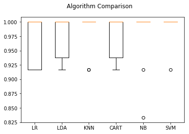
Since K-Nearest Neighbors was the best classifier on the training set we run that one over the validation set and get the out-of-sample predictions.

There is a little bit of machine learning jargon baked in this next part:

1. The ‘confusion matrix’ is pretty much what it sounds like. It’s a table showing the observations that were misclassified. There doesn’t seem to me to be a lot of agreement regarding a standardized definition of the ‘confusion matrix.’ Pythons scikit-learn confusion_matrix method just prints the observations that were misclassified…but I’ve seen some applications where the matrix for a binary classification (output on the [0,1] scale) is a 4 X 4 with the number of points correctly classified as 0 in the (1,1) cell, number of observations classified as 1 but were really 0 in the (1,2) cell, number of observations classified as 0 but were really 1 in the (2,1) cell, and number of observations correctly classified as 1 in the (2,2) cell.

2. The accuracy score is just the percent of the validation set that was correctly predicted. Our validation set is 30 observations and there were 3 errors so the accuracy score is 0.9 because 90% of the observations in the validation set were correctly classified.

3. The classification report has 3 parts for each grouping in the data:

• precision: this is the ability of the classifier not to label as positive a sample which was negative, $\frac{tp}{tp+fp}$, where $tp$ is true positive and $fp$ is false positive.
• recall: the ability of the classifier to find all positive samples, $\frac{tp}{tp+fn}$, where $fn$ is false negative
• f1-score: the harmonic mean of precision and recall.
• support is the number of observations in the validation set belonging to each class.

#-------------------------------------------------------
# Make predictions on validation dataset
knn = KNeighborsClassifier()
knn.fit(X_train, Y_train)
predictions = knn.predict(X_validation)
print(accuracy_score(Y_validation, predictions))
print(confusion_matrix(Y_validation, predictions))
print(classification_report(Y_validation, predictions))

#--------------------------------------------------------

0.9
[[ 7  0  0]
 [ 0 11  1]
 [ 0  2  9]]
                 precision    recall  f1-score   support

    Iris-setosa       1.00      1.00      1.00         7
Iris-versicolor       0.85      0.92      0.88        12
 Iris-virginica       0.90      0.82      0.86        11

    avg / total       0.90      0.90      0.90        30

The classification report tells us that:

1. all 7 of the Iris-Setosa samples in the validation set were correctly classified
2. of the 12 Iris-versicolor sample in the validation set, one was incorrectly classified as Iris-virginica and two Iris-virginica samples were classified as Iris-versicolor
3. of the 11 Iris-virginica, two were incorrectly classified as Iris-versicolor and one Iris-versicolor was incorrectly classified as Iris-verginica.